Chapter 13 Tag likelihoods
This section explores a range of tag-recovery likelihoods that have been used in the literature. A simple tag recapture model is used in a simulation to explore how well different likelihoods estimate movement parameters under a range of over-dispersion assumptions. The tag-recapture model ignores age and models number of tagged fish from a release event denoted by \(k\) over three regions indexed by \(r\) for \(n_t\) discrete time-steps. \(T^k_{r,t}\) denotes the number of tagged fish from release event \(k\) in region \(r\) and time step \(t\). The model applies the following processes between time-steps.
\[\begin{align*} T^k_{r,t} & = T^k, \quad t = 0\\ T^k_{r,t + 1} & = T^k_{r,t} e^{-Z_t}, \quad t > 0\\ Z_t & = M + F_t \\ \boldsymbol{T}^k_{t + 1} & = \boldsymbol{T}^k_{t + 1} \boldsymbol{M} \end{align*}\] where, \(T^k\) is the initial nunmber of tag releases for release event \(k\), \(\boldsymbol{T}^k_{t + 1} = (T^k_{1,t + 1},\dots, T^k_{n_r,t + 1})\) is a vector of numbers of tagged fish across all regions and \(\boldsymbol{M}\) is a \(n_r \times n_r\) movement matrix. This assumes each region has the same fishing mortality in each time-step.
Likelihoods
For all possible tag-recovery events indexed by \(m\) (where \(m = \{r,t\}\) i.e., has an implied region and time-step dimension) the tag-recapture model derives expected tag-recoveries. In this case, any time or region that has any fishing mortality rate is considered a possible tag-recovery event. All the likelihoods in the following sections use the same derivation for expected tag-recoveries, which follows
\[ N^k_{m} = T^k_{r,t} \left(1 - e^{-Z_t}\right) \frac{F_t}{Z_t}, \quad m = \{r,t\} \ . \]
Poisson
The Poisson is the simplest likelihood, which was explored by Hilborn (1990). It assumes
\[ N^k_{m} \sim \mathcal{Poisson}(\widehat{N}^k_{m}) \, \]
with the total log-likelihood contribution evaluating the Poisson log-likelihood over all possible release and recovery events (\(\sum\limits_k\sum\limits_m\))
Negative Binomial
A similar likelihood to the Poisson is the Negative Binomial which was explored by Hanselman et al. (2015). This is a more flexible likelihood as it allows for over dispersion, through an additional estimable parameter denoted by \(\phi\)
\[ N^k_{m} \sim \mathcal{NB}(\widehat{N}^k_{m}, \widehat{\phi}) \, \]
with the total log-likelihood contribution evaluating the Negative binomial log-likelihood over all possible release and recovery events (\(\sum\limits_k\sum\limits_m\))
Multinomial:release conditioned
The release conditioned multinomial likelihood was explored by Polacheck et al. (2006) and subsequently by Vincent, Brenden, and Bence (2020) & D. R. Goethel, Legault, and Cadrin (2014). This treats all recovery events plus an additional not-recovered event as a multinomial distributed event.
\[ \boldsymbol{N}^k \sim \mathcal{Multinomial}\left(\widehat{\boldsymbol{\theta}}^k\right) \] where, \(\boldsymbol{N}^k\) is the vector of tag-recoveries for all possible recovery events (\(n_m\)) plus an additional not-recovered event. \[ \boldsymbol{N}^k = (N^k_1, N^k_2, \dots, N^k_{n_m}, N^k_{NR}) \] where, \(N^k_{NR}\) represents the not recovered category and is \(N^k_{NR} = T^k - \sum\limits_m^{n_m} N^k_m\), where \(T^k\) is the initial number of tags released for event \(k\). \(\widehat{\boldsymbol{\theta}}^k\) is a vector of proportions that sum to one, with the same dimensions as \(\boldsymbol{N}^k\) and is calculated as,
\[ \widehat{\theta}^k_m = \frac{\widehat{N}^k_{m}}{T^k}, \quad \forall \ m \in (1, \dots,n_m) \] where, again \(T^k\) is the initial number of tags released for event \(k\). The proportions for the not recaptured group is calculated as, \[ \widehat{\theta}^k_{NR} = 1 - \sum_m^{n_m} \widehat{\theta}^k_m \]
Recapture conditioned
The multinomial which is recapture conditioned follows that described by Vincent, Brenden, and Bence (2020) but based on the original work of McGarvey and Feenstra (2002). This likelihood evaluates the probability of recapturing a tagged fish in a certain region among all possible regions for a given release event and time-period.
\[ \boldsymbol{N}^k_t \sim \mathcal{Multinomial}\left(\widehat{\boldsymbol{\theta}}_t^k\right) \] where, \(\boldsymbol{N}^k_t\) is the vector of tag-recoveries in all regions (\(n_m\)) for release event \(k\) and time period \(t\) \[ \boldsymbol{N}^k_t = (N^k_{1,t}, N^k_{2,t}, \dots, N^k_{n_r,t}) \] and model predicted proportions \[ \widehat{\boldsymbol{\theta}}_t^k = (\widehat{\theta}^k_{1,t}, \widehat{\theta}^k_{2,t}, \dots, \widehat{\theta}^k_{n_r,t}) \] and,
\[ \widehat{\theta}^k_{r,t} = \frac{\widehat{N}^k_{r,t}}{\sum\limits_r \widehat{N}^k_{r,t}} \]
The literature (McGarvey and Feenstra 2002; Vincent, Brenden, and Bence 2020) often describes the log likelihood as
\[ ll = \sum_k\sum_y\sum_r log(\widehat{\theta}^k_{r,t}) \times N^k_{r,t} \]
Simple simulation
To explore these likelihoods are very simple simulation was setup to see how well each likelihood could estimate elements of \(\boldsymbol{M}\) under different levels of over-dispersion. The simulation assumes all tags encountered where reported (100% reporting rate) and both natural mortality and fishing mortality are known without error. The only estimated parameters were \(\boldsymbol{M}\) and \(\phi\) when the negative binomial likelihood was explored.
Tag recovery observations were all simulated using the negative binomial likelihood with varying over-dispersion parameters.
The following is some R-code that was used to generate operating model values for
set.seed(123)
n_y = 5
n_regions = 3
M = 0.13
F_y = rlnorm(n = n_y, log(0.2), 0.6)
Z_y = F_y + M
S_y = exp(-Z_y)
# make up some random movement matrix
move_matrix = matrix(0, ncol = n_regions, nrow = n_regions)
diag(move_matrix) = c(0.7, 0.5, 0.6)
move_matrix = move_matrix + rnorm(n = n_regions * n_regions, 0.1,0.05)
move_matrix = sweep(move_matrix, MARGIN = 1, STATS = rowSums(move_matrix), FUN = "/")
## seed tag releases
tag_release_by_region = rep(1000, n_regions)
n_release_events = n_regions
## Calculate tag-partition
tags_partition_by_release_event = array(0, dim = c(n_regions, n_y + 1, n_release_events))
expected_tag_recoveries  = tag_recovery_obs = array(0, dim = c(n_regions, n_y, n_release_events))
for(r in 1:n_release_events)
  tags_partition_by_release_event[r,1,r] = tag_release_by_region[r]
for(y in 1:n_y) {
  for(rel_event in 1:n_release_events) {
    ## ageing and F
    tags_partition_by_release_event[,y + 1, rel_event] =
      tags_partition_by_release_event[,y,rel_event] * S_y[y]
    ## Movement
    tags_partition_by_release_event[,y + 1, rel_event] =
      tags_partition_by_release_event[,y + 1, rel_event] %*% move_matrix
  }
}

## Create tag-recovery expected values
for(rel_event in 1:n_regions) {
  expected_tag_recoveries[,,rel_event] =
    sweep(tags_partition_by_release_event[ ,2:(n_y + 1),rel_event], MARGIN = 2, STATS =  F_y / Z_y * (1 - S_y), FUN = "*")
}
The following code chunk assumes tags_partition_by_release_event is the same among simulations, but uses the negative binomial with a range of over-dispersion parameters to simulate tag-recoveries for n_sim times. We explore Relative error (RE) and mean square error (MSE) for the different likelihood choices.
n_sim = 500
## Populate TMB objects
data = list()
data$n_y = n_y
data$n_regions = n_regions
data$M = M
data$F_y = F_y
data$tag_likelihood = 0 ## Poisson
data$tag_recovery_obs = tag_recovery_obs
data$number_of_tags_released = tag_release_by_region
data$movement_transformation = 0 ## simplex, can use the logistic transformation as well
## starting values
est_parameters = list()
start_matrix = matrix(0, ncol = n_regions, nrow = n_regions)
diag(start_matrix) = c(0.95, 0.95, 0.95)
start_matrix = start_matrix + rnorm(n = n_regions * n_regions, 0.02,0.0001)
## force to sum = 1
start_matrix = sweep(start_matrix, MARGIN = 1, STATS = rowSums(start_matrix), FUN = "/")

est_parameters$transformed_movement_pars = matrix(NA, nrow = n_regions - 1, ncol = n_regions)
for(i in 1:n_regions)
  est_parameters$transformed_movement_pars[,i] = simplex(start_matrix[i,])
est_parameters$ln_phi = log(1)
## don't estimate phi parameter unless Negative binomial
na_map = fix_pars(par_list = est_parameters, pars_to_exclude = "ln_phi")

OM_mat = melt(move_matrix)
colnames(OM_mat) = c("From", "To","proportion")
OM_mat$type = "OM"
############################################
## over_diserpsion_investication
## what happens when we simualte from
## negative binomial with different
## over-dispersion parameters
############################################
over_dispersion_params = c(0.1, 0.2, 0.3, 0.5, 1, 10)
n_sim = 500
# use the simplex
data$movement_transformation = 0
sim_data_info = NULL
complete_df = NULL
for(over_ndx in 1:length(over_dispersion_params)) {
this_dispersion = over_dispersion_params[over_ndx]
full_move_df = NULL;
temp_proportion_zeros_sim_data = temp_variance_sim_data = c()
for(sim in 1:n_sim) {
## keep expected values the same among simulations
for(rel_event in 1:n_release_events) {
for(y in 1:n_y) {
for(r in 1:n_regions) {
tag_recovery_obs[r,y,rel_event] = rnbinom(n = 1, mu = expected_tag_recoveries[ r,y,rel_event], size = this_dispersion)
}
}
}
## summarise number of zeros and variance of observed data
temp_proportion_zeros_sim_data = c(temp_proportion_zeros_sim_data, sum(tag_recovery_obs == 0));
temp_variance_sim_data = c(temp_variance_sim_data, var(tag_recovery_obs));
## save data
data$tag_recovery_obs = tag_recovery_obs
## Poisson
data$tag_likelihood = 0
est_obj <- MakeADFun(data, est_parameters, map = na_map, DLL="SimpleTagEstimator", silent = T)
est_obj$env$tracepar = F
opt_poisson = nlminb(est_obj$par, est_obj$fn, est_obj$gr, control = list(iter.max = 10000, eval.max = 10000))
poisson_rep = est_obj$report(opt_poisson$par)
sd_poisson = sdreport(est_obj)
## Multinomial release conditioned
data$tag_likelihood = 1
est_obj <- MakeADFun(data, est_parameters, map = na_map, DLL="SimpleTagEstimator", silent =T)
opt_multi_release = nlminb(est_obj$par, est_obj$fn, est_obj$gr, control = list(iter.max = 10000, eval.max = 10000))
multi_release_rep = est_obj$report(opt_multi_release$par)
sd_multi_release = sdreport(est_obj)
## Multinomial recapture conditioned
data$tag_likelihood = 2
est_obj <- MakeADFun(data, est_parameters,map = na_map, DLL="SimpleTagEstimator", silent = T)
opt_multi_recap = nlminb(est_obj$par, est_obj$fn, est_obj$gr, control = list(iter.max = 10000, eval.max = 10000))
multi_recap_rep = est_obj$report(opt_multi_recap$par)
sd_multi_recap = sdreport(est_obj)
## recapture conditioned
data$tag_likelihood = 3
est_obj <- MakeADFun(data, est_parameters,map = na_map, DLL="SimpleTagEstimator", silent = T)
opt_recap = nlminb(est_obj$par, est_obj$fn, est_obj$gr, control = list(iter.max = 10000, eval.max = 10000))
recap_rep = est_obj$report(opt_recap$par)
sd_recap = sdreport(est_obj)
## Negative binomial
data$tag_likelihood = 4
est_obj <- MakeADFun(data, est_parameters, DLL="SimpleTagEstimator", silent = T)
opt_nb = nlminb(est_obj$par, est_obj$fn, est_obj$gr, control = list(iter.max = 10000, eval.max = 10000))
nb_rep = est_obj$report(opt_nb$par)
sd_nb = sdreport(est_obj)
## reformat movement estimates
pois_mat = melt(poisson_rep$movement_matrix)
pois_mat$RE = (pois_mat$value - OM_mat$proportion) / OM_mat$proportion * 100
pois_mat$SE = (OM_mat$proportion - pois_mat$value)^2
pois_mat$type = "Poisson"
pois_mat$sim = sim
recap_mat = melt(recap_rep$movement_matrix)
recap_mat$RE = (recap_mat$value - OM_mat$proportion) / OM_mat$proportion * 100
recap_mat$SE = (OM_mat$proportion - recap_mat$value)^2
recap_mat$type = "Recapture"
recap_mat$sim = sim
multi_release_mat = melt(multi_release_rep$movement_matrix)
multi_release_mat$RE = (multi_release_mat$value - OM_mat$proportion) / OM_mat$proportion * 100
multi_release_mat$SE = (OM_mat$proportion - multi_release_mat$value)^2
multi_release_mat$type = "Multinomial Release"
multi_release_mat$sim = sim
nb_mat = melt(nb_rep$movement_matrix)
nb_mat$RE = (nb_mat$value - OM_mat$proportion) / OM_mat$proportion * 100
nb_mat$SE = (OM_mat$proportion - nb_mat$value)^2
nb_mat$type = "Negative Binomial"
nb_mat$sim = sim
full_move_df = rbind(full_move_df, rbind(pois_mat, recap_mat, multi_release_mat, nb_mat))
}
prop_obs_zero = temp_proportion_zeros_sim_data / (dim(data$tag_recovery_obs)[1] * dim(data$tag_recovery_obs)[2] * dim(data$tag_recovery_obs)[3])
tmp_df = data.frame(avg_proportion_zero = mean(prop_obs_zero), avg_var = mean(temp_variance_sim_data), over_dispersion_param = this_dispersion)
sim_data_info = rbind(sim_data_info, tmp_df)
full_move_df$over_dispersion_param = this_dispersion
complete_df = rbind(complete_df, full_move_df)
}
colnames(complete_df) = c("From", "To","proportion", "RE", "SE", "type", "sim", "over_dispersion_param")| avg_proportion_zero | avg_var | over_dispersion_param |
|---|---|---|
| 0.603 | 10135.388 | 0.1 |
| 0.417 | 5552.975 | 0.2 |
| 0.296 | 4003.506 | 0.3 |
| 0.176 | 2321.719 | 0.5 |
| 0.068 | 1505.669 | 1.0 |
| 0.002 | 561.667 | 10.0 |
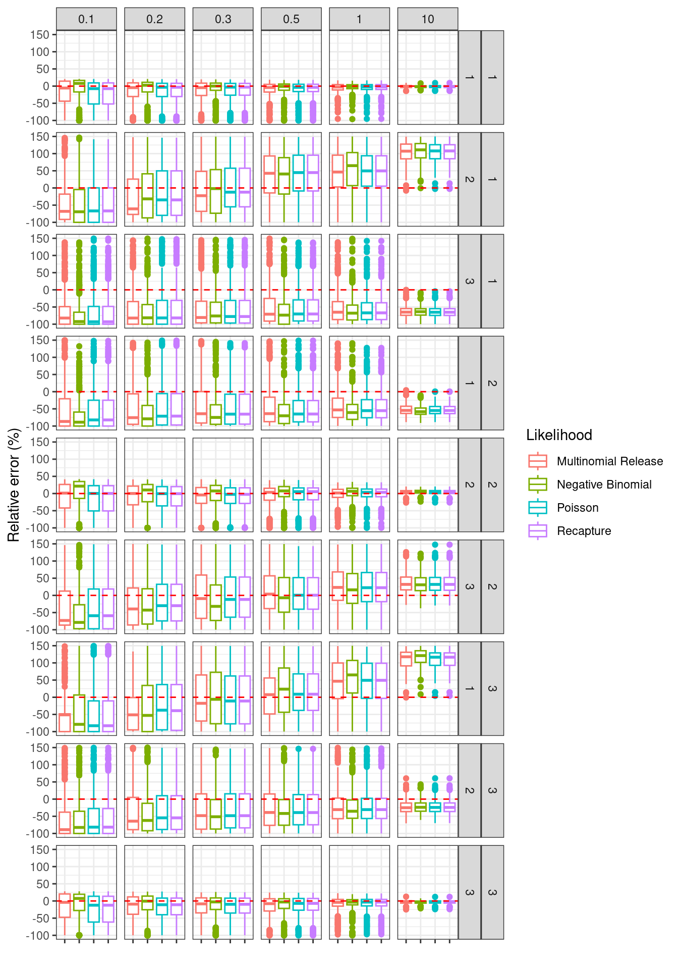
Figure 13.1: Relative error in movement parameters. Columns are overdispersion values for simulated data. GGplot facets are movement matrix elemen combinatons
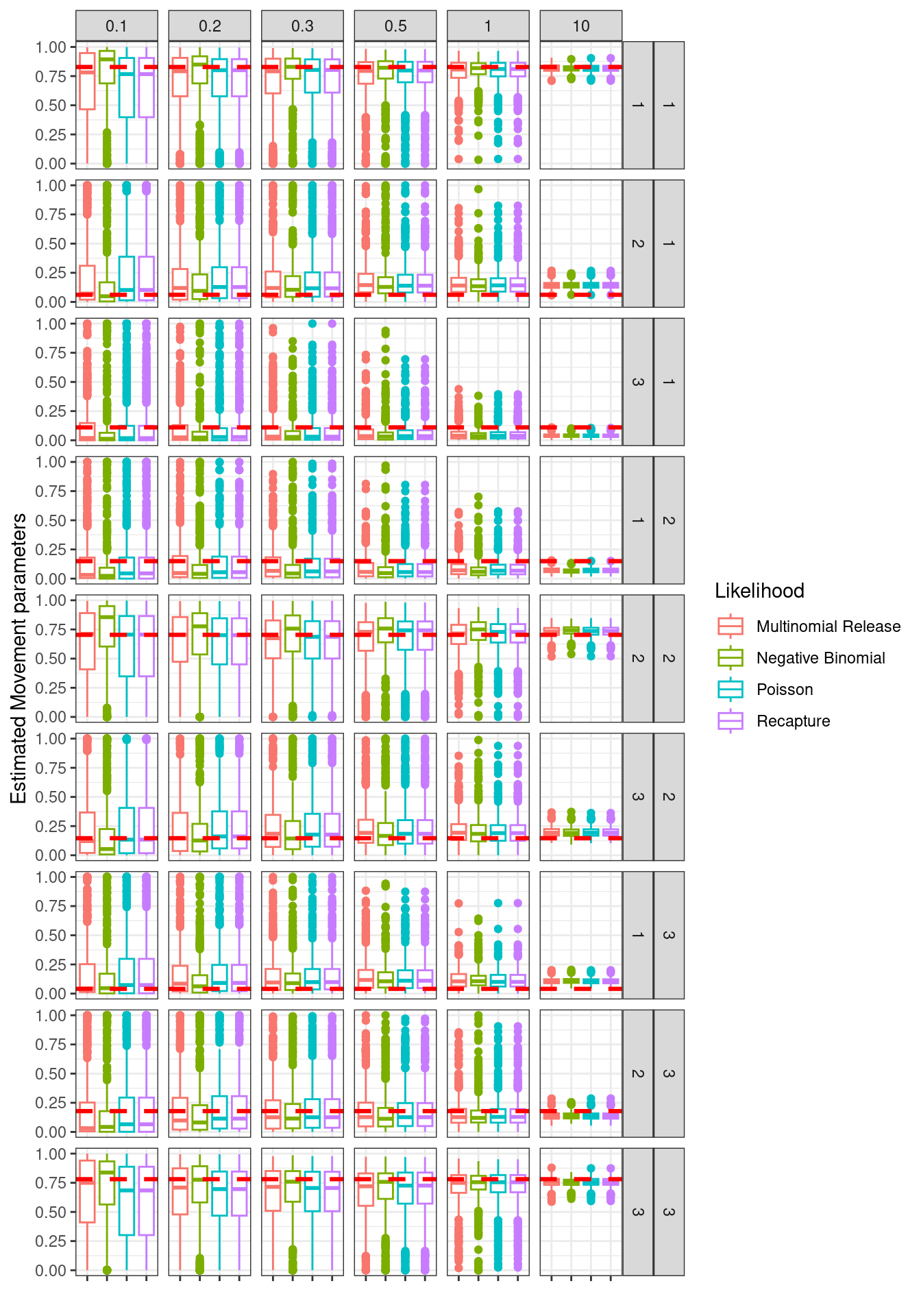
Figure 13.2: Estimated movement parameters, red line is true value. Columns are overdispersion values for simulated data. GGplot facets are movement matrix elemen combinatons
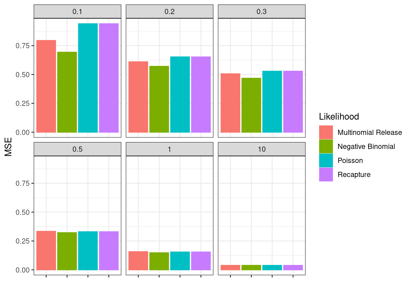
Figure 13.3: Mean squared error (MSE) over all simulations and estimated parameters.