Chapter 17 Fishing mortality approaches
The current Alaskan sablefish stock assessment (Chapter 3) estimates annual fishing mortality values for each gear \(g\) denoted by \(F^g_{y}\). This parametersation poses to potential problems when considering future assessment models and spatial models. The first is, the number of parameters will increase as the number of gears increase. The fishery is currently going through a transformation whereby there is a switch from longline to pots. The second consideration is how to set this up in a spatially explicit model where catch have an added spatial dimension. There are two alternative approaches to the current approach which treat \(F\) as a derived quantity rather than an estimable parameter. The first is to use Newton Raphson method to solve for \(F^g_{y}\). This is the recommended approach in Stock Synthesis (Methot Jr and Wetzel 2013), termed the “hybrid” approach. The previous two methods assume the Baranov catch equation for mortality (Baranov 1918). An alternative is to assume Popes discrete formulation (Pope 1972) which uses exploitation proportions (sometimes called harvest rates or fishing pressure) and has a closed form solution.
A good general overview on these methods can be found in Branch (2009). They describe and compared the continuous Baranov catch equation (Baranov 1918) with Pope’s discrete formulation (Pope 1972). Arguments for using the continuous case is that \(M\) and \(F\) occur simultaneously, also with the continuous case, \(F\) allows for multiple event encounters, this is assuming a fleet has the same selectivity and availability, that a fish that escapes one net can be caught in another. In contrast, the discrete formulation only allows a fish to be caught or escape from an instantaneous event. I have tried to summarize the benefits of the continuous equation in the following list,
- Allows the entire population to be caught (not sure this is that relevant)
- Allows simultaneous \(M\) and \(F\), no need to worry about order of operations. From a coding/practical perspective this is quite attractive. Once you have an F and M you can easily derive all mid-mortality quantities. Where as using a \(U\) approach you need save the population before and after to interpolate to derive mid-mortality quantities.
- The magnitude of \(F\) effects composition data, where as in the discrete case, composition is independent of the magniture of \(U\).
- Allows for multiple catch events of an individual
- Can fit to catch observations thus allows for uncertainty in catches. In practice the uncertainty/variance on catch is very small i.e., coeffecient of variations ranging from 0.01 to 0.1. This essentially states catch is observed with high confidence and in my opinion isn’t that much different to saying catch is known exactly. Note often this high precision on observed catch is needed in order to make the \(F\)’s identifiable. This high precision also muddies the “degrees of freedom” for the model. Although the \(F\)’s look like independent and free parameters they are heavily constrained by the assumptiosn on observed catch variance.
The arguments for the discrete approximation is that there is an analytical solution for \(U\) and so is fast to calculate expected catch, where as \(F\) has to be either solved numerically or estimated as a free parameter (as mentioned earlier).
Chris Francis’s wrote a response to this paper (Francis 2010) where he argues the discrete formulation does not preclude the multiple encounters and that only the data can truly tell us which catch equation is the best one to use.
- Need to make a point about how there may be Automatic differentiation issues with the \(U\) approach. Because there is an
if(U > 0.99)which can cause a fork in the chain rule which can equal a coding nightmare.
The relationship between \(F\) (Instantaneous fishing mortality) and \(U\) exploitation rate for a simple scenario (single fishery) is illustrated in the following R code.
exploitation_rates = seq(0,0.8,by = 0.02)
## calculate F given a U
fishing_mortalites = -log(1 - exploitation_rates)
## back calculate U given a F
# 1 - exp(-fishing_mortalites)
The objective of this simulation
- Is the method efficient i.e., no loss of speed.
- Is the method numerically stable (No NaNs during optimization), particularly under high fishing pressure
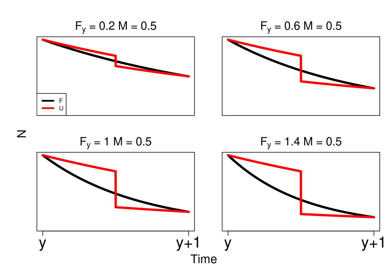
Figure 17.1: Illustration of how mortality is applied to an age cohort continuously over time (y).
Set up a simulation
To explore the above described methods a simple simulation was conducted using a simple age-structured stock assessment operating model. The model assumed 15 seperate fisheries all with a common selectivity. The purpose was to check that the derived methods were reliable (provided unbiased stock quantities) and that they are computationally efficient.
bio_params = list(
  ages = 1:20,
  L_inf = 58,
  K = 0.133,
  t0 = 0,
  M = 0.15,
  a = 2.08e-9, ## tonnes
  b = 3.5,
  m_a50 = 6.3,
  m_ato95 = 1.2,
  sigma = 0.6,
  h = 0.85,
  sigma_r = 0.6,
  R0 = 8234132,
  plus_group = 1 # 0 = No, 1 = Yes
)

other_params = list(
  s_a50 = 3.6,
  s_ato95 = 2,
  s_q = 0.2,
  f_a50 = 5,
  f_ato95 = 2,
  ssb_prop_Z = 0.5,
  survey_prop_Z = 0.5,
  survey_age_error = c(0.5, 0.4),  ## sd, rho (ignored if iid)
  fishery_age_error = c(0.5, 0.4),  ## sd, rho (ignored if iid)
  survey_bio_cv = c(0.1)
)

ages = bio_params$ages
max_age = max(bio_params$ages)
n_years = 30
years = (2020 - n_years + 1):2020
n_ages = length(ages)
## annual fishing mortality
start_F = c(rlnorm(10, log(seq(from = 0.05, to = 0.2, length = 10)), 0.1), rlnorm(10, log(0.13), 0.1), rlnorm(10, log(0.07), 0.1))
recruit_devs = log(rlnorm(n_years, -0.5 * bio_params$sigma_r * bio_params$sigma_r, bio_params$sigma_r))

length_at_age = vonbert(bio_params$ages, bio_params$K, bio_params$L_inf, bio_params$t0)
fishery_ogive = logis(bio_params$ages, other_params$f_a50, other_params$f_ato95)
survey_ogive = logis(bio_params$ages, other_params$s_a50, other_params$s_ato95)
mat_age = logis(bio_params$ages, bio_params$m_a50, bio_params$m_ato95)
weight_at_age = bio_params$a * length_at_age^bio_params$b

## observation temporal frequency
survey_year_obs = years
survey_ages = 1:20
fishery_year_obs = years
fishery_ages = 1:20
## simulate data
set.seed(123)
sim_data = ASM_obj$simulate(complete = T)
## Build AD TMB functions
start_pars = ran_start_vals()
est_model_est_F = MakeADFun(sim_data, true_pars, DLL= "SimpleAgestructuredModelMultiFs", map = na_map, silent = T)
sim_data$F_method = 1
sim_data$F_iterations = 4
est_model_hybrid_F = MakeADFun(sim_data, true_pars, DLL= "SimpleAgestructuredModelMultiFs", map = na_map_hybrid, silent = T)
## optimise
opt_model_est_F = nlminb(est_model_est_F$par, est_model_est_F$fn, est_model_est_F$gr, control = list(iter.max = 10000, eval.max = 10000))
opt_model_hybrid_F = nlminb(est_model_hybrid_F$par, est_model_hybrid_F$fn, est_model_hybrid_F$gr, control = list(iter.max = 10000, eval.max = 10000))
## look at the number of iterations used to solve
opt_model_hybrid_F$iterations## [1] 187opt_model_est_F$iterations## [1] 697## get reports =
rep_est_hybrid = est_model_hybrid_F$report(est_model_hybrid_F$env$last.par.best)
rep_est_F = est_model_est_F$report(est_model_est_F$env$last.par.best)
plot(TMB_data$years, rep_est_hybrid$ssb[-1], type = "l", lwd = 3, xlab = "Year", ylab = "SSB", ylim = c(0,46000))
lines(TMB_data$years, rep_est_F$ssb[-1], type = "l", lwd = 3, lty = 2, col = "purple")
lines(TMB_data$years, sim_data$ssb[-1], type = "l", lwd = 4, lty = 3, col = "red")
legend("topright", col = c("black", "purple", "red"), legend = c("Hybrid", "Est F", "OM"), lwd = 3)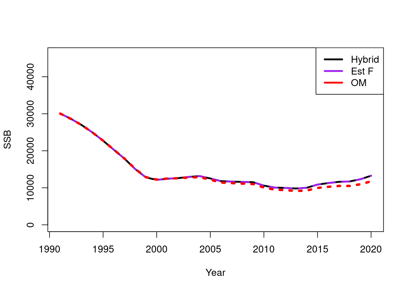
est_F_bench = benchmark(obj = est_model_est_F, n = 1000)
hybrid_F_bench = benchmark(obj = est_model_hybrid_F, n = 1000)
est_F_bench
## elapsed
## template.likelihood 0.895
## template.gradient 1.737hybrid_F_bench## elapsed
## template.likelihood 2.394
## template.gradient 4.811ben_est_F <- benchmark(obj = est_model_est_F, n=20,expr=expression(do.call("optim",obj)))
ben_hybrid_F <- benchmark(obj = est_model_hybrid_F, n=20,expr=expression(do.call("optim",obj)))
ben_est_F## elapsed
## do.call("optim", obj) 15.217ben_hybrid_F## elapsed
## do.call("optim", obj) 12.935These results have highlighted the following
- Both the Free \(F\) and hybrid estimate very similar model quantities i.e., SSB’s and F’s
- The Free \(F\) method is much faster on average for a single gradient calculation and function call compared to the hybrid method
- However, the hybrid method requires less iterations due to there being less estimated parameters. For this simulation where we assumed 15 fisheries both optimised in similar amounts of time
Appendix - Hybrid approach
The hybrid fishing mortality process uses the methods and algorithms applied in Stock Synthesis (Methot Jr and Wetzel 2013). The descriptions below are heavily based on the text describing this approach in the Appendix of (Methot Jr and Wetzel 2013).
This process begins by calculating popes discrete approximation, and then converts this to Baranov fishing mortality coefficients. A tuning algorithm is then done to tune these coefficients to match input catch nearly exactly, rather than the full Baranov approach.
Total mortality, denoted by \(Z_{a,y,s,r}\) for sex \(s\), region \(r\), age \(a\) and year \(y\) will hereby be denoted by \(Z_{a,y,s}\) i.e., drop the region index. This is because mortality rates are calculated independently (in isolation) among regions (NOTE consider parallelising this in the model).
\[\begin{equation*} Z_{a,y,s} = M_{a,y,s} + \sum\limits_{f} S^g_{y,s} F^g_y \end{equation*}\]
where, \(M_{a,s}\) is the natural mortality rate, \(F^g_y\) is fishing mortality and \(S^g_{a,s}\) is the selectivity.
The hybrid fishing mortality method allows the \(F\) values to be “tuned” to match input catch nearly exactly, rather than estimating them as free model parameters. The process begins by calculating mid year exploitation rate using Pope’s approximation. This exploitation rate is then converted to an approximation of the Baranov continuous \(F\). The \(F\) values for all fisheries operating in that year and region are then tuned over a set number of iterations (f_iterations) to match the observed catch for each fishery with its corresponding \(F\). Differentiability is achieved by the use of Pope’s approximation to obtain the starting value for each \(F\) and then the use of a fixed number of tuning iterations, typically 4. Tests from Stock Synthesis have shown that modelling \(F\) as hybrid versus \(F\) as a parameter has trivial impact on the estimates of the variances of other model derived quantities.
The hybrid method calculates the harvest rate using the Pope’s approximation then converts to an approximation of the corresponding F as:
\[\begin{align} V^g_{y} &= \sum\limits_s\sum\limits_a N_{a,y,s} \exp\left(-\delta_t M_{a,s}\right) \nonumber \\ \tilde{U}^g_{y} &= \frac{C^g_{y}}{V^g_{y} + 0.1 C^g_{y}}\\ j^g_{y} &= \left(1 + \exp \left(30 (\tilde{U}^g_{y} - 0.95) \right)\right)^{-1}\\ U^g_{y} &= j^g_{y} \tilde{U}^g_{y} + 0.95 (1 - j^g_{y} )\\ \tilde{F}^g_{y} &= \frac{-\log\left(1 - U^g_{y}\right)}{\delta_t} \end{align}\]
where, \(C^{g}_y\) is the observed catch, \(\delta_t\) is the duration of the period of observation within the year. In most situations where the entire catch has been observed in a time-step. This should be one. \(V^g_{y}\) is partway vulnerable biomass and \(\tilde{F}^g_{y}\) is the initial \(F\).
The formulation above is designed so that high exploitation rates (above 0.95) are converted into an F that corresponds to a harvest rate of close to 0.95, thus providing a more robust starting point for subsequent iterative adjustment of this F. The logistic joiner, \(j\), is used at other places in Stock Synthesis to link across discontinuities.
The tuning algorithm begins by setting \(F^g_{y} = \tilde{F}^g_{y}\) and repeating the following algorithm f_iteration times.
\[ \widehat{C}_{a,y,s} = \sum\limits_g {F}^g_{y}S^g_{a,s} N_{a,y,s}\bar{w}_{a,y,s} \lambda^*_{a,y,s} \]
where, \(\lambda^*_{a,y,s}\) denotes the survivorship and is calculated as:
\[\begin{equation} \lambda^*_{a,y,s} = \frac{1 - \exp\left(-\delta_t Z_{a,y,s} \right) }{Z_{a,y,s}} \tag{17.1} \end{equation}\]
Total fishing mortality is then adjusted over several fixed number of iterations (typically four, but more in high F and multiple fishery situations). The first step is to calculate the ratio of the total observed catch over all fleets to the predicted total catch according to the current F estimates. This ratio provides an overall adjustment factor to bring the total mortality closer to what it will be after adjusting the individual \(F\) values.
\[ \widehat{C}_{y} = \sum\limits_g \sum\limits_s\sum\limits_a {F}^g_{y}\left(S^g_{a,s} N_{a,y,s}\right) \lambda^*_{a,y,s} \]
This is different from Equation A.1.25 in the Appendix of (Methot Jr and Wetzel 2013). They include \(Z_{a,y,s}\) in the denominator when describing \({F}^g_{y}\), I think this is a typo error because \(Z_{a,y,s}\) is already included in the denominator when calculating \(\lambda^*_{a,y,s}\) (see Equation (17.1)).
\[ Z^{adj}_y = \frac{\sum\limits_g C^g_{y}}{\widehat{C}_{y}} \]
The total mortality if this adjuster was applied to all the Fs is then calculated:
\[ Z^*_{a,y,s} = M_{a,s} + Z^{adj}_y \left(Z_{a,y,s} -M_{a,s} \right) \]
\[ \lambda^*_{a,y,s} = \frac{1 - \exp\left(-\delta_t Z^*_{a,y,s} \right) }{Z^*_{a,y,s}} \]
The adjusted mortality rate is used to calculate the total removals for each fishery, and then the new \(F\) estimate is calculated by the ratio of observed catch to total removals, with a constraint to prevent unreasonably high \(F\) calculations (max_f):
\[\begin{align*} \tilde{V}^g_{y} &= \sum\limits_s\sum\limits_a \left(N_{a,y,s} \bar{w}_{a,y,s}S^g_{a,s} \right)\lambda^*_{a,y,s} \\ F^{g*}_{y} &= \frac{C^g_{y}}{\tilde{V}^g_{y} + 0.0001}\\ j^{g*}_{y} &= \left(1 + \exp \left(30 (F^{g*}_{y} - 0.95 F_{max}) \right)\right)^{-1}\\ \end{align*}\]
where, \(F_{max}\) is a user defined maximum fishing mortality f_max. The \(F\) at the end of each tuning iteration follows:
\[ F^g_{y} = j^{g*}_{y} F^{g*}_{y} + \left(1 - j^{g*}_{y}\right)F_{max} \]
After the tuning algorithm removals at age, and other derived quantities are recorded. The final total mortality is updated \[ Z_{a,y,s} = M_{a,s} + \sum\limits_{g} S^g_{a,s} F^g_{y} \]
This process generates catch at age and sex for each year (and region) (\(\widehat{C}^g_{a,y,s}\)) which can be accessed by process_removals observations. Numbers at age are calculated as
\[ \widehat{C}^g_{a,y,s} = \frac{F^g_{a,s,y}}{Z_{a,y,s}} N_{a,y,s} \exp\left(-Z_{a,y,s}\right) \]
Total catch is the summed over all sexes and age
\[ \widehat{C}^g_{y} = \sum\limits_s\sum\limits_a \widehat{C}^g_{a,y,s} \bar{w}_{a,y,s} \]
where \(\bar{w}_{a,y,s}\) is the mean weight