Chapter 12 Estimating age-based movement
To explore estimating age-based movement a simple age-based tagging process model was coded, which assumed
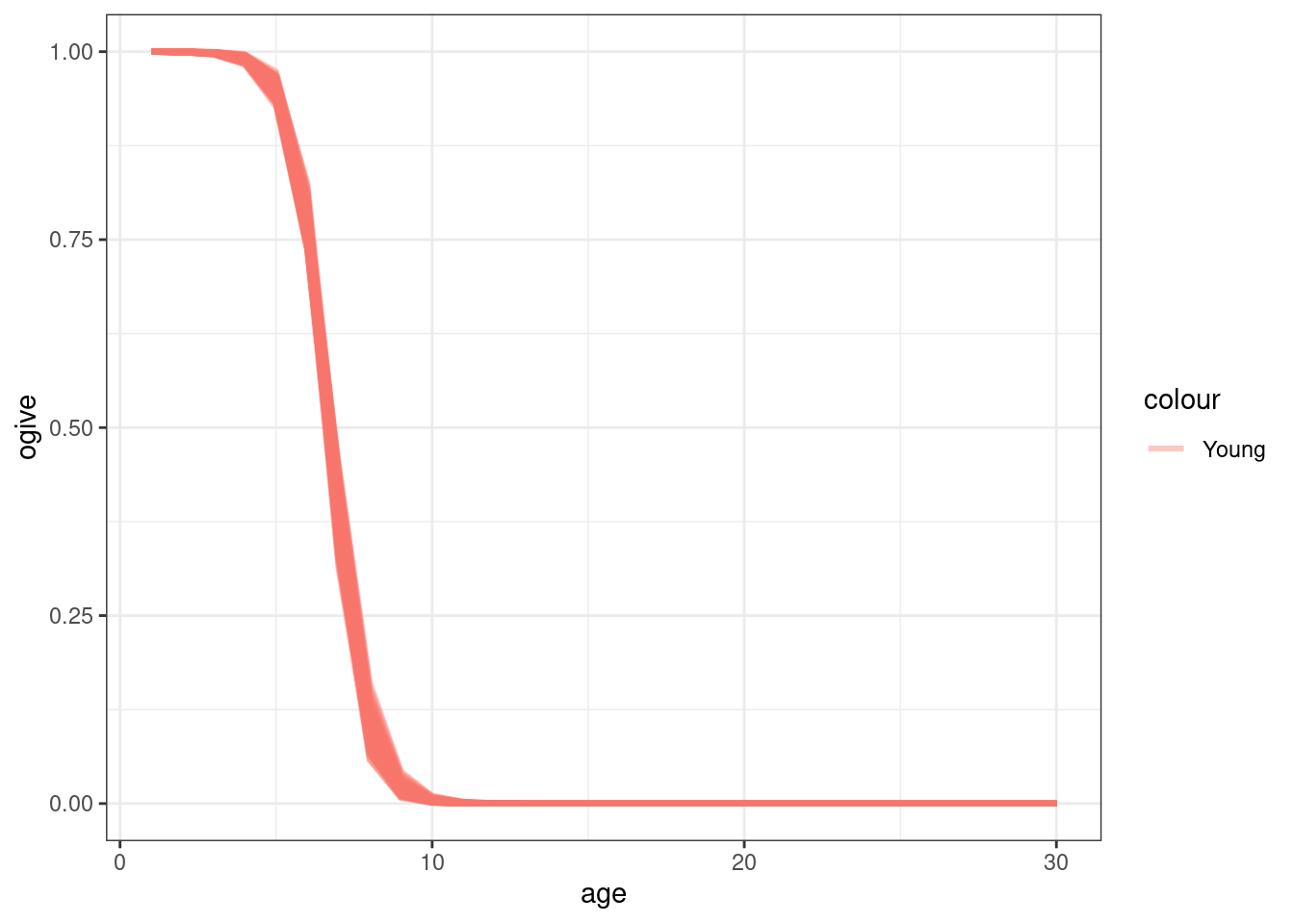
\[\begin{align*} T^k_{a, r,t} & = T_a^k, \quad t = 0\\ T^k_{a, r,t + 1} & = T^k_{a, r,t} e^{-M}, \quad t > 0\\ \boldsymbol{T}^k_{a, t + 1} & = \boldsymbol{T}^k_{a, t + 1} (1 - S^o_a) \boldsymbol{M}^y + \boldsymbol{T}^k_{a, t + 1} S^o_a \boldsymbol{M}^o \end{align*}\] where, \(T_a^k\) is the initial number of tag releases for release event \(k\) and age \(a\), \(\boldsymbol{T}^k_{a, t + 1}\) is a matrix of numbers of tagged fish across all regions from release event \(k\) and age \(a\), \(\boldsymbol{M}^y\) is a \(n_r \times n_r\) movement matrix for young fish and \(\boldsymbol{M}^o\) is the movement matrix for older fish. \(S^o_a\) is a movement based logistic ogive that determines what proportion of age-cohorts move based on \(\boldsymbol{M}^o\) and \((1 - S^o_a)\) indicates what proportion of age-cohorts move based on \(\boldsymbol{M}^y\). The age-based selectivity is parametersised as a logistic ogive with estimable parameters \(a_{50}\) (age at which \(S^o_a = 0.5\)) and \(a_{to95}\) (difference age when \(S^o_a = 0.5\) and \(S^o_a = 0.95\)),
\[ S^o_a = \frac{1}{1 + 19^{(a_{50} - a) / a_{to95}}} \]
Generating age-based observations
First attempt
The first attempt was to use the age based ogive to split our observed tag recoveries by age (\(N^k_{a, r,t}\)) into the young tag recoveries (\({Y}^k_{r,t}\)) and old tag recoveries (\({O}^k_{r,t}\)) and assume these are Poisson distributed.
\[\begin{align*} \widehat{Y}^k_{r,t} & = \sum_a \widehat{T}^k_{a, r,t}(1 - \widehat{S}^o_a) \\ \widehat{O}^k_{r,t} & = \sum_a \widehat{T}^k_{a, r,t} \widehat{S}^o_a \\ {Y}^k_{r,t} & = \sum_a N^k_{a, r,t}(1 - \widehat{S}^o_a) \\ {O}^k_{r,t} & = \sum_a N^k_{a, r,t} \widehat{S}^o_a \\ {Y}^k_{r,t} &\sim \mathcal{Poisson}\left(\widehat{Y}^k_{r,t}\right)\\ {O}^k_{r,t} &\sim \mathcal{Poisson}\left(\widehat{O}^k_{r,t}\right) \end{align*}\]
\(\widehat{Y}^k_{r,t}\) expected tag recoveries for young fish, and \(\widehat{O}^k_{r,t}\) is the expected tag recoveries for old fish, and \(N^k_{a, r,t}\) is the observed tag-recovery by age.
The problem with this approach is we are using model estimated quantities (\(\widehat{S}^o_a\)) to classify observed values as young and old, which is a no no. Simulations also showed that we could not estimate both parameters of \(\widehat{S}^o_a\).
Second attempt
The second attempt was to assume the age-structure was multinomial as,
\[\begin{align*} \widehat{\theta}^k_{a, r,t} &= \frac{\widehat{T}^k_{a, r,t}}{\sum_a \widehat{T}^k_{a, r,t}}\\ N^k_{a, r,t} &\sim \mathcal{Multinomial}\left(\widehat{\theta}^k_{a, r,t}\right)\\ \end{align*}\] with the effective sample size being the sum of the observations. This treatment of the data resulted in much more robust estimation of movement rates and all parameters of the movement ogive.
Simulation summary
The following section is code and plots from running the three following simulations,
- Simulate tag-recoveries with the Poisson distribution, estimate \(\boldsymbol{M}^y\) and \(\boldsymbol{M}^o\) with \(S^o_a\) fixed at values assumed in the OM
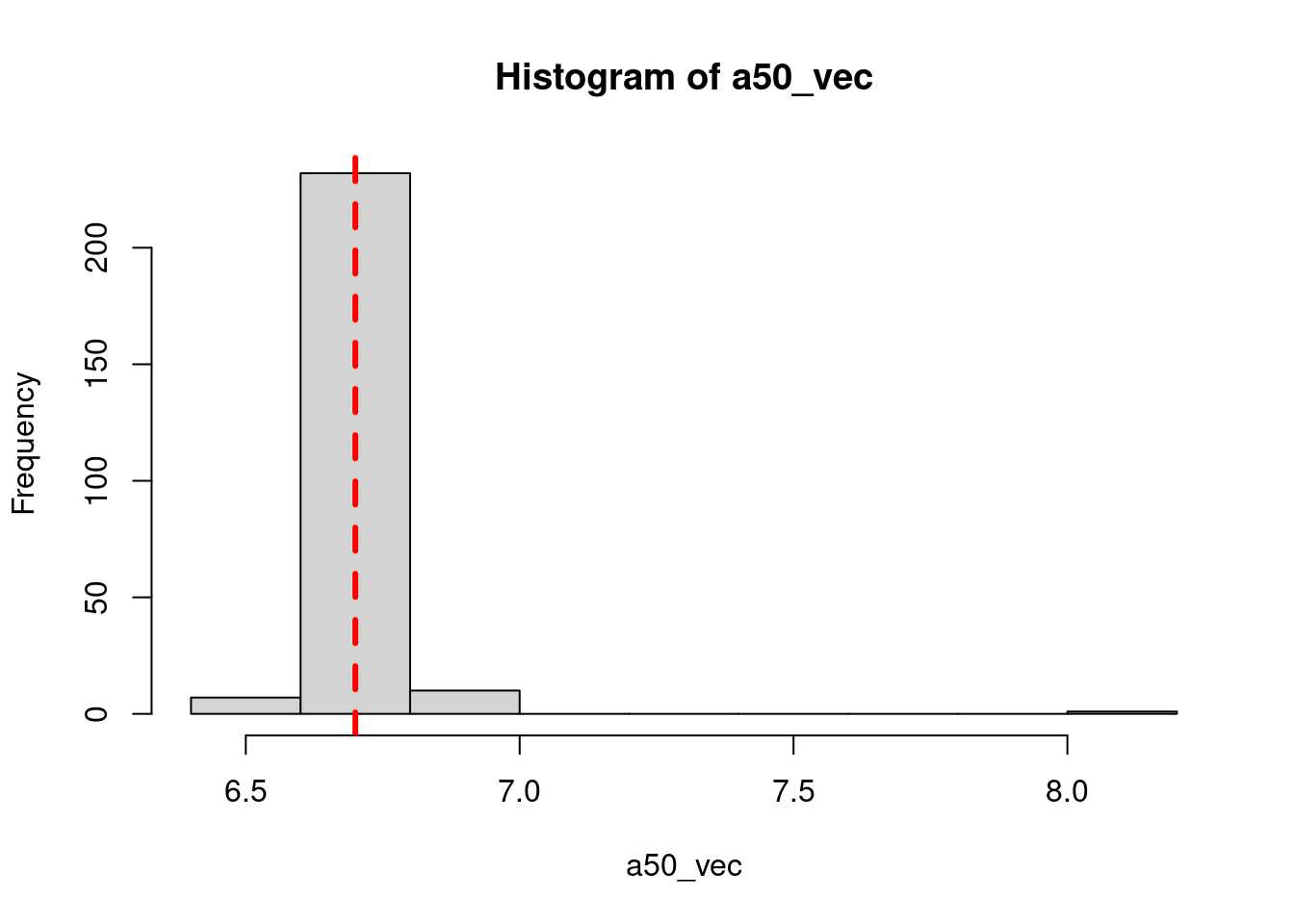
- Simulate tag-recoveries with the Poisson distribution, estimate \(\boldsymbol{M}^y\), \(\boldsymbol{M}^o\), and \(a_{50}\) from \(S^o_a\), with \(a_{to95}\) fixed at the value assumed in the OM
- Simulate tag-recoveries with the Poisson distribution, estimate \(\boldsymbol{M}^y\), \(\boldsymbol{M}^o\), \(a_{50}\), and \(a_{to95}\)
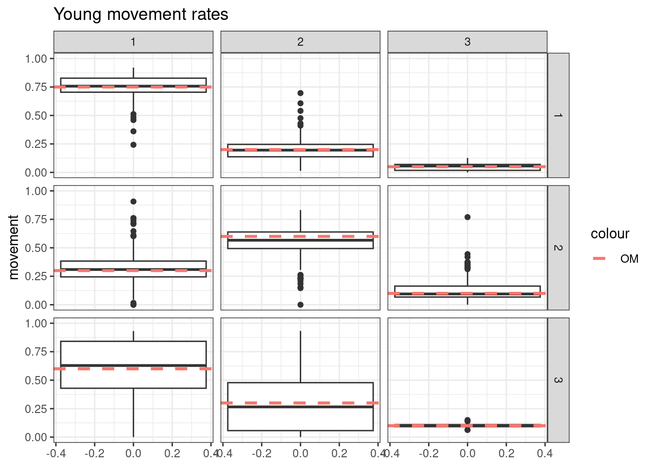
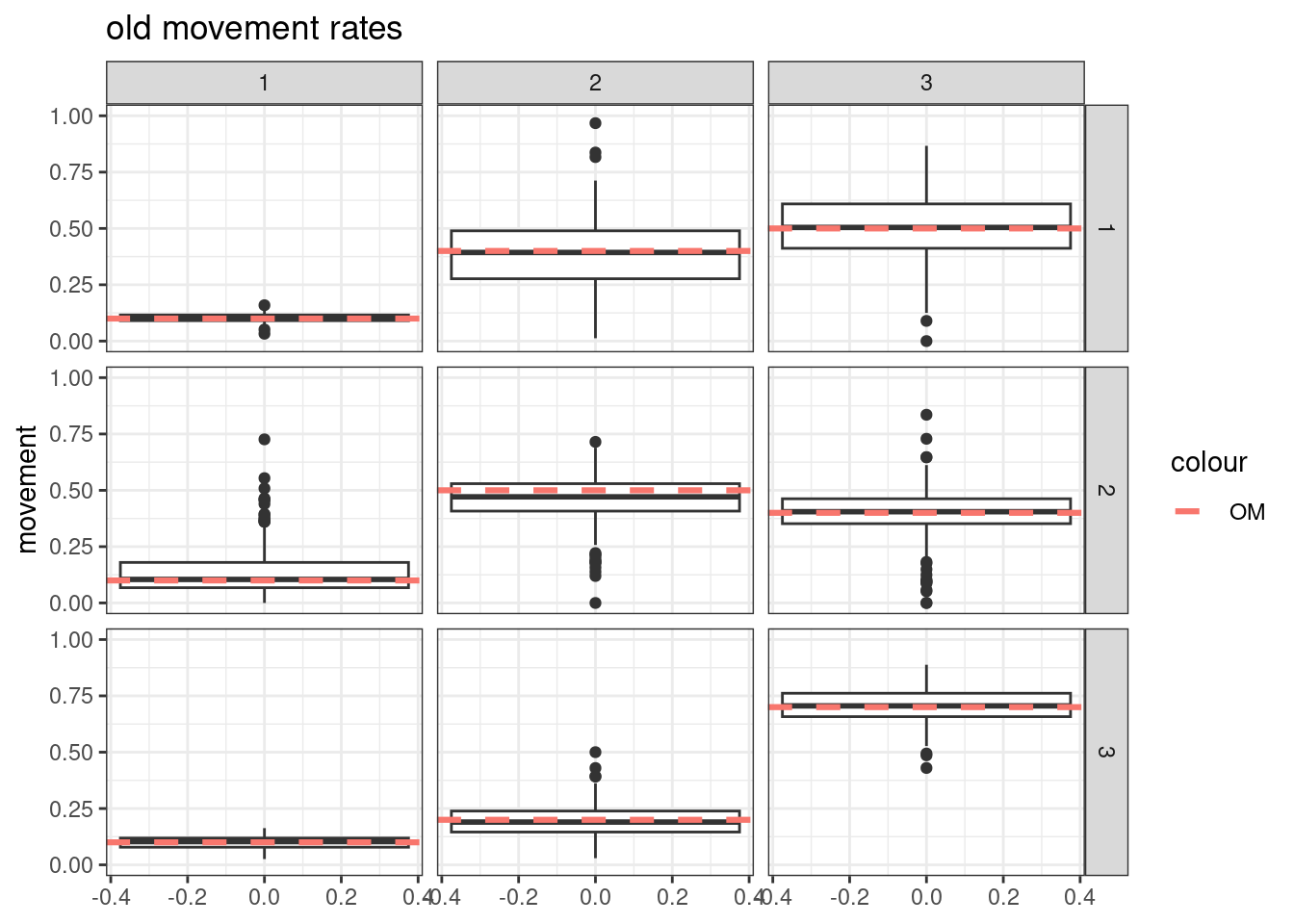
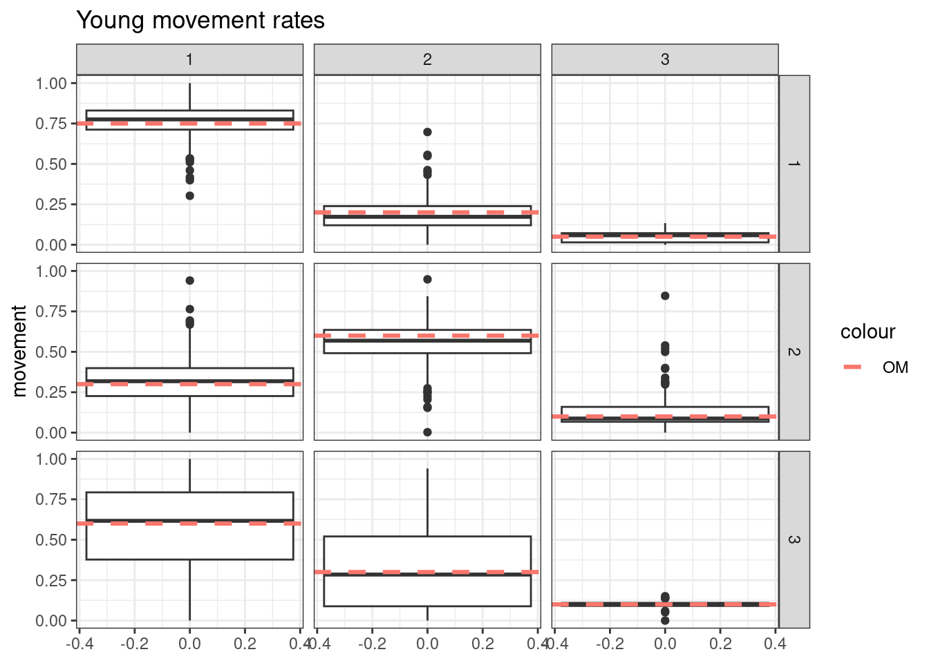
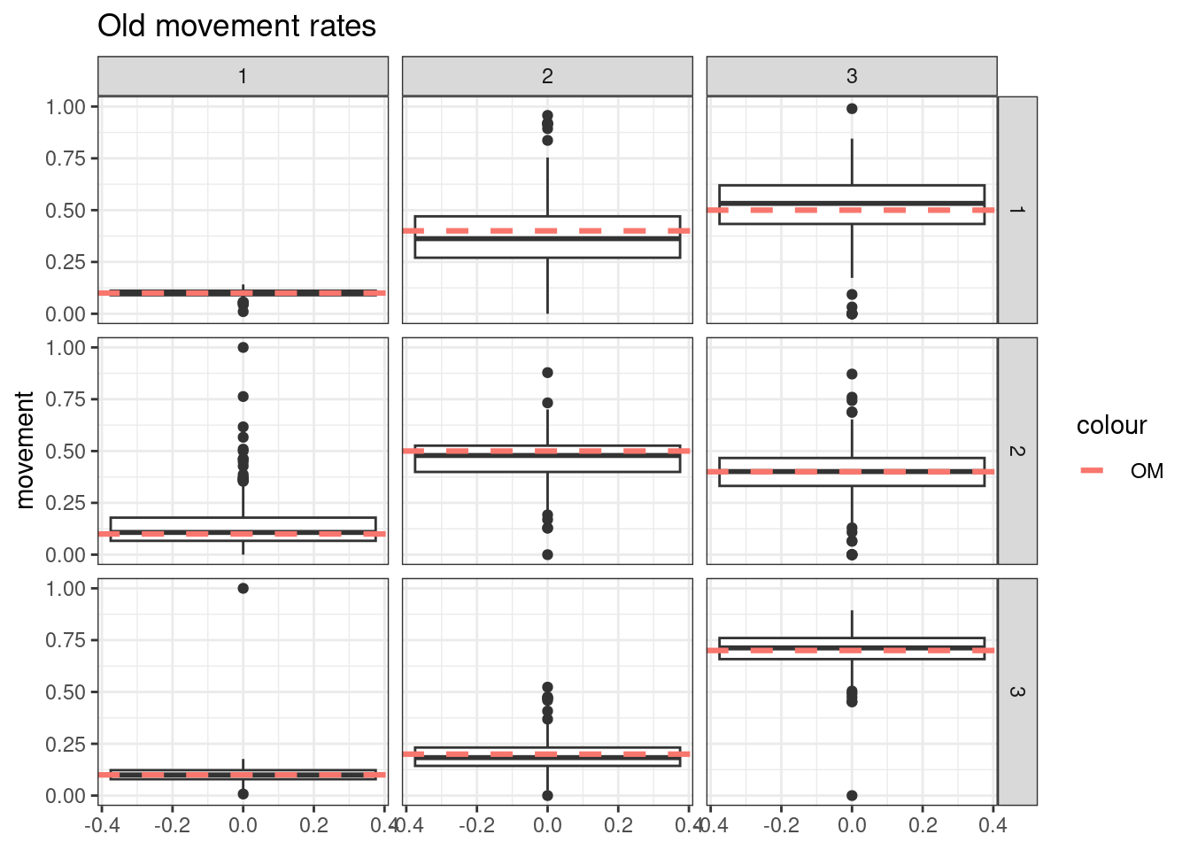
Results from these simulations using the first likelihood attempt show when \(S^o_a\) is correctly specified you can estimate both \(\boldsymbol{M}^y\) and \(\boldsymbol{M}^o\) well (caveats = good data and correct likelihood). This was also true when estimating just the \(a_{50}\) parameter when \(a_{to95}\) is specified correctly. However, when trying to estimate both movement matrices and both \(a_{50}\) and \(a_{to95}\) we get parameter estimating problems. With both parameters running to lower bounds. Interestingly the \(\boldsymbol{M}^y\) is estimated well, but \(\boldsymbol{M}^o\) has large biases. This same result occurs when specifying \(a_{to95}\) at a low value (almost knife edge) and just estimating \(a_{50}\), results not shown here.
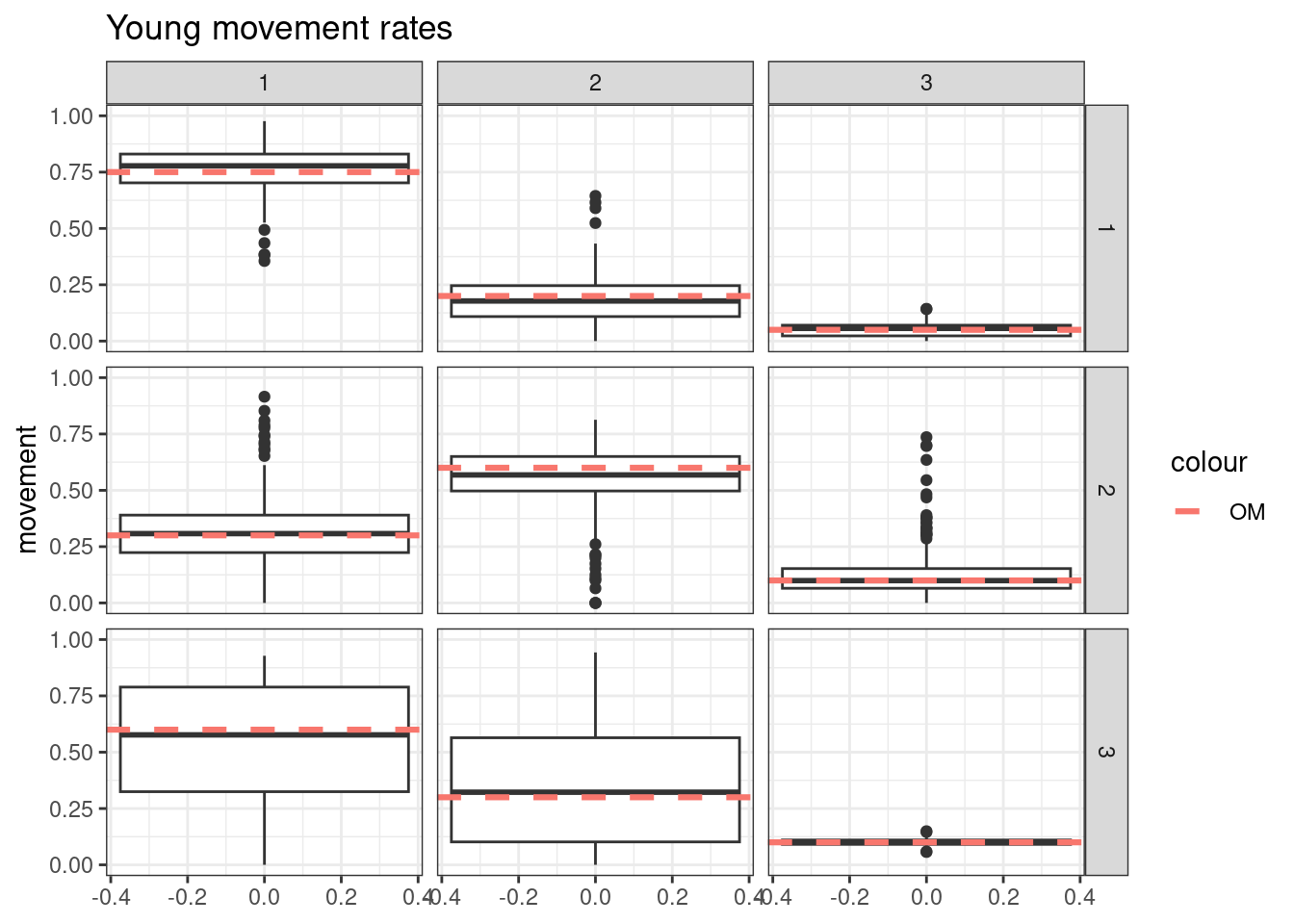
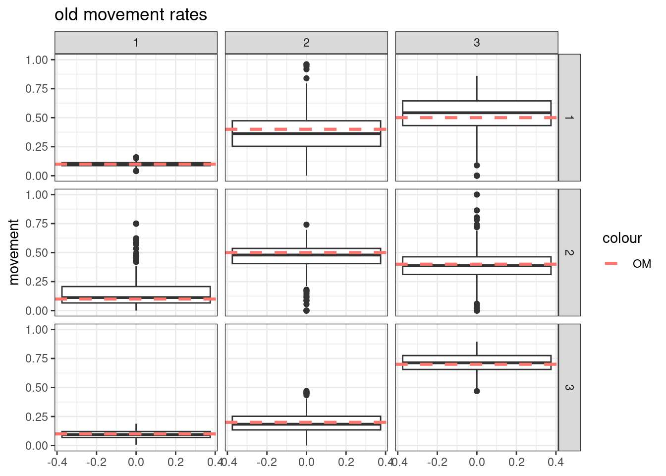
Results from these simulations using the second likelihood attempt show under all three simulations we can get resonable estimates of both movement matriceis and age-based movement ogive parameters.
Setup simulations
M = 0.12
R0 = 20000
ages = 1:30
n_regions = 3
young_move_matrix = old_move_matrix = matrix(rnorm(n_regions * n_regions, 10, 3), nrow = n_regions, ncol = n_regions)
## young movement
## encouraged to stay closer to region 1
young_move_matrix[1,1] = 0.75
young_move_matrix[1,2] = 0.2
young_move_matrix[1,3] = 0.05
young_move_matrix[2,1] = 0.3
young_move_matrix[2,2] = 0.6
young_move_matrix[2,3] = 0.1
young_move_matrix[3,1] = 0.6
young_move_matrix[3,2] = 0.3
young_move_matrix[3,3] = 0.1
## old movement
## encouraged to stay closer to region 3
old_move_matrix[1,1] = 0.1
old_move_matrix[1,2] = 0.4
old_move_matrix[1,3] = 0.5
old_move_matrix[2,1] = 0.1
old_move_matrix[2,2] = 0.5
old_move_matrix[2,3] = 0.4
old_move_matrix[3,1] = 0.1
old_move_matrix[3,2] = 0.2
old_move_matrix[3,3] = 0.7
true_young_molten_move = melt(young_move_matrix)
true_old_molten_move = melt(old_move_matrix)
colnames(true_young_molten_move) = colnames(true_old_molten_move) = c("From", "To", "movement")
## age based movement ogive
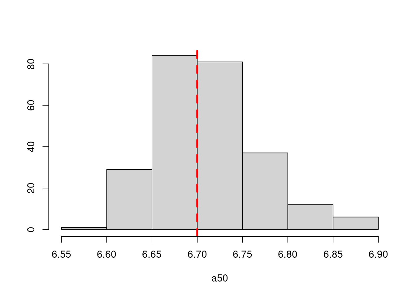
a50_move = 6.7
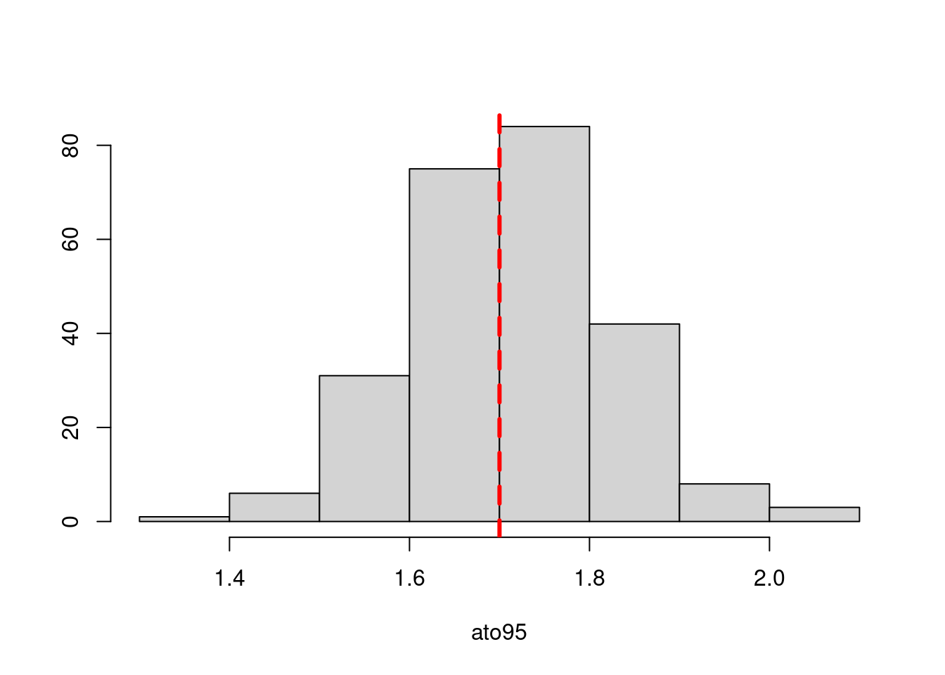
a95_move = 1.7
old_age_based_movement = logis(ages, a50_move, a95_move)
young_age_based_movement = 1 - old_age_based_movement
init_N_age = calculate_initial_numbers_at_age_age_based_movement(n_regions, n_ages = length(ages), R0, old_movement_matrix = old_move_matrix, young_movement_matrix = young_move_matrix, age_based_movement_ogive = young_age_based_movement, natural_mortality =rep(M, length(ages)))
data = list()
data$initial_age_tag_releases = t(init_N_age)
data$natural_mortality = M
data$n_years = 5
data$n_ages = length(ages)
data$n_regions = n_regions
data$ages = ages
data$tag_recovery_obs = array(100, dim = c(data$n_ages, n_regions, n_regions, data$n_years))
data$a50_bounds = c(3, 15)
data$tag_likelihood_type = 1 ## multinomial
parameters = list()
parameters$logisitic_a50_movement = logit_general(a50_move, data$a50_bounds[1], data$a50_bounds[2])
parameters$ln_ato95_movement = log(a95_move)
parameters$transformed_movement_pars_young = array(0, dim = c(n_regions - 1, n_regions))
parameters$transformed_movement_pars_old = array(0, dim = c(n_regions - 1, n_regions))
for(r in 1:n_regions) {
parameters$transformed_movement_pars_young[,r] = simplex(young_move_matrix[r, ])
parameters$transformed_movement_pars_old[,r] = simplex(old_move_matrix[r, ])
}
test_obj <- MakeADFun(data = data, parameters = parameters, DLL="SimpleAgeBasedMovement")## Constructing atomic D_lgamma