Chapter 7 Tagging data exploration
Since 1972 there have been approximately 400 000 sablefish tagged in Alaska waters, of which over 38 500 have been recovered. Although there is extensive and long term tagging data, this information is not currently directly included in the stock assessment (D. Goethel et al. 2021).
Historical publications investigating movement of Alaskan sablefish include Heifetz and Fujioka (1991), Hanselman et al. (2015)
Data grooming
| rule | events | events_removed | relative_events |
|---|---|---|---|
| Init | 36159 | 0 | 0.00 |
| Duplicated recovery id | 36104 | 1085 | -2.92 |
| negative time-at-liberty recovery id | 35884 | 220 | -0.61 |
| NA lat and long | 35884 | 0 | 0.00 |
| Tag type: AB, BK, JU, SA, SB | 30986 | 4898 | -13.65 |
| Area: BS, AI, EGOA, WGOA, CGOA | 22535 | 8451 | -27.27 |
| Gear recovery: 901, 902 | 19214 | 3321 | -14.74 |
| Exclude survey recoveries | 16805 | 2409 | -12.54 |
| Release code: 623, 901, 902, 915 | 13267 | 3538 | -21.05 |
| Release depth > 150 | 10850 | 2417 | -18.22 |
| rule | events | events_removed | relative_events |
|---|---|---|---|
| Init | 395146 | 0 | 0.00 |
| Duplicated recovery id | 390768 | 4378 | -1.11 |
| NA lat and long | 390767 | 1 | 0.00 |
| Tag type: AB, BK, JU, SA, SB | 337603 | 53164 | -13.61 |
| Area: BS, AI, EGOA, WGOA, CGOA | 276427 | 61176 | -18.12 |
| Release code: 623, 901, 902, 915 | 241525 | 34902 | -12.63 |
| Release depth > 150 | 202563 | 38962 | -16.13 |
Exploratory analysis of the tag data
Figure 7.1 shows the spatial distribution of both releases and recaptures, which both have fairly broad spatial distributions which is a good attribute. Figure 7.2 shows the number of recoveries by gear method and year, this highlights a major drop off in recoveries from the Longline gear with no other gear has picked up in. This will have to be discussed with the wider team. In particular, what years to consider this data to be informative.
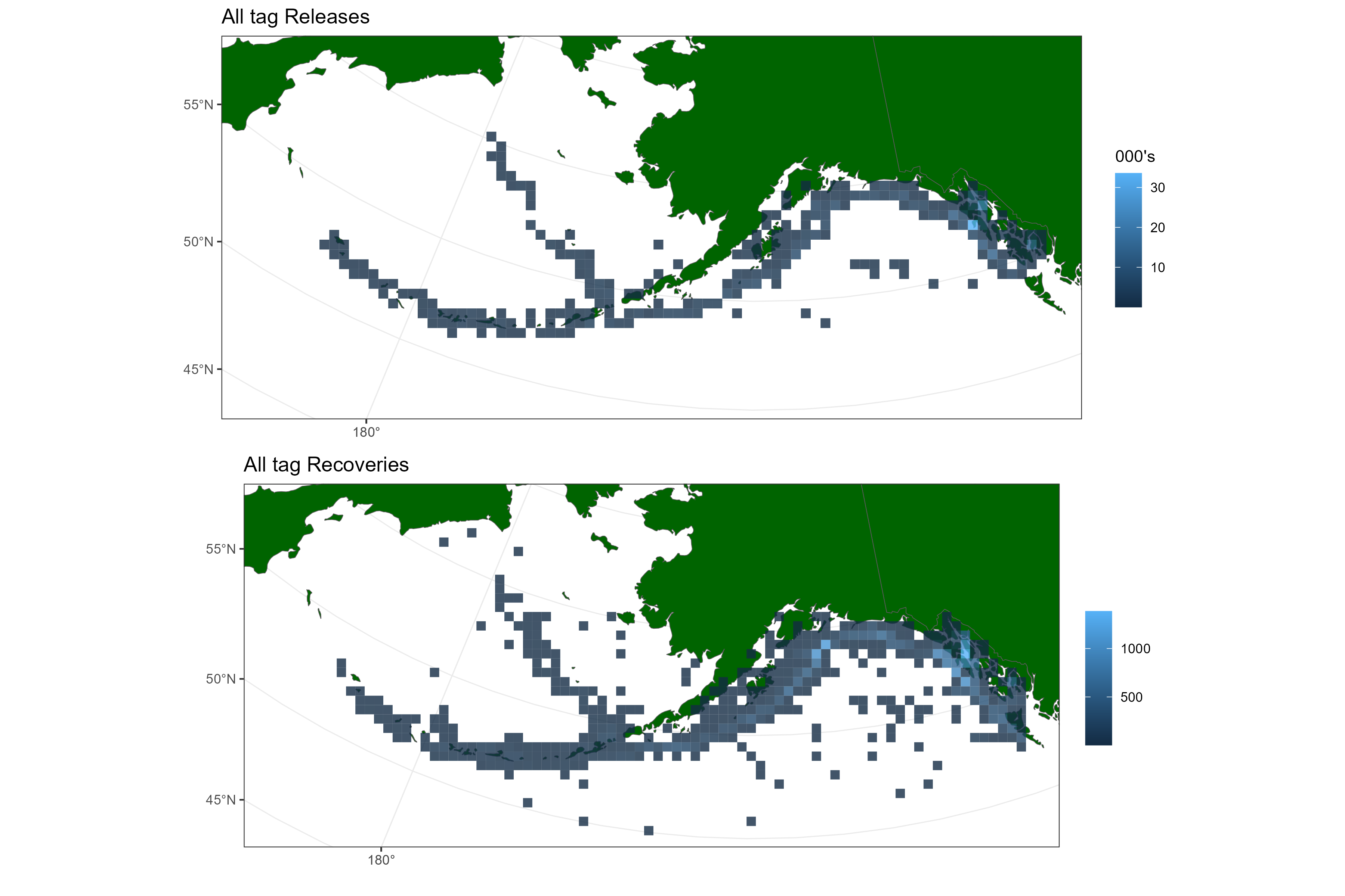
Figure 7.1: Tag releases and recoveries pooled over all years
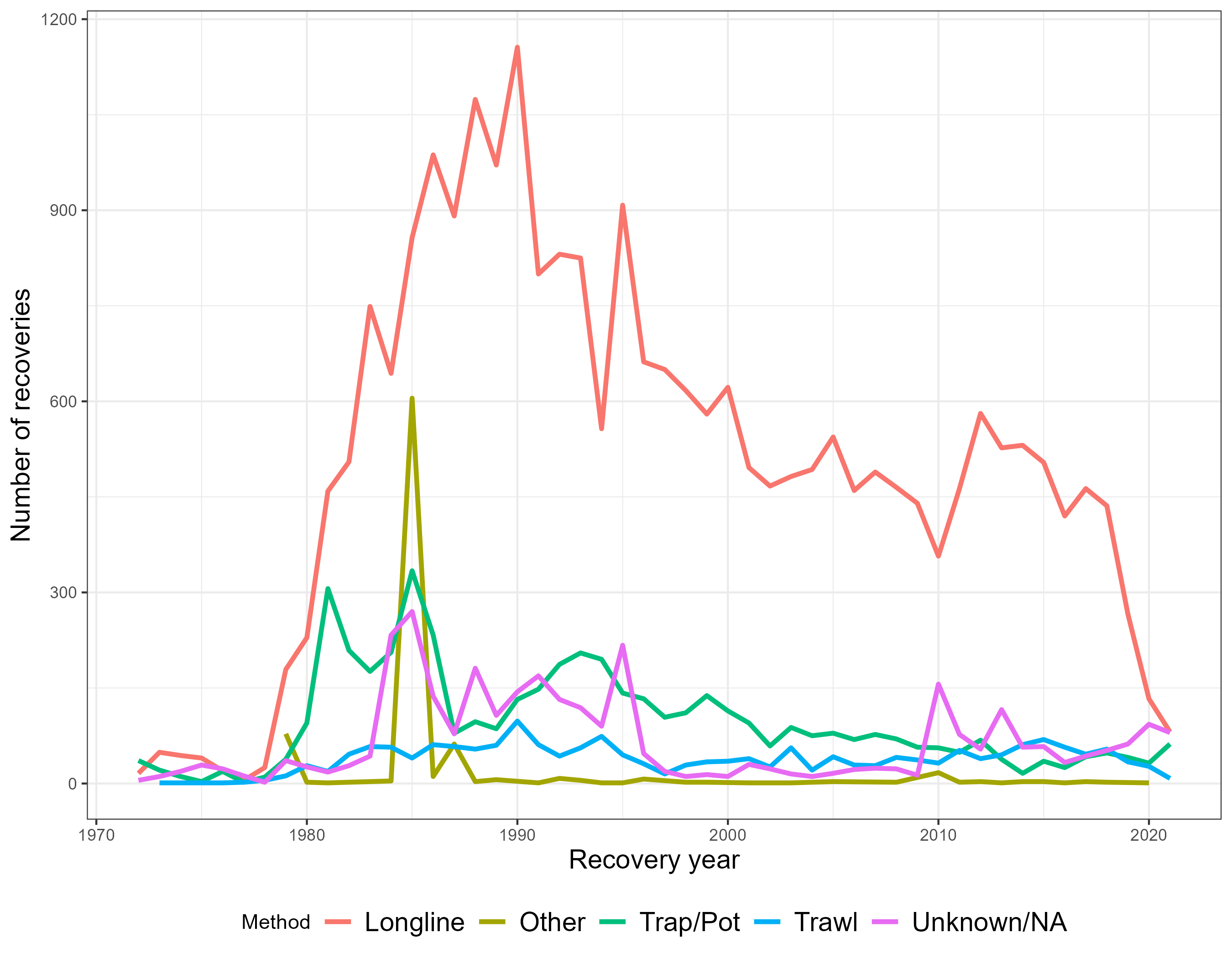
Figure 7.2: Recovered fish by gear type and year
One thing of note is the number of tag-recaptures outside of the stock boundaries, shown in Figure 7.3.
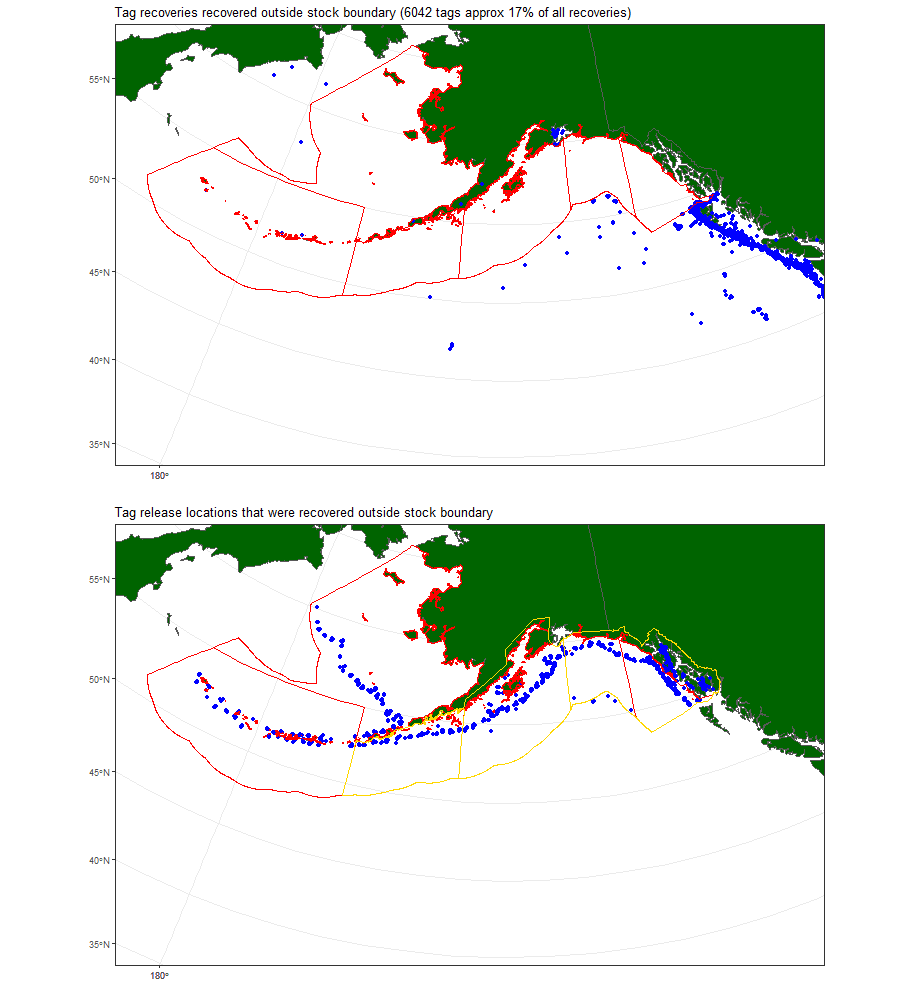
Figure 7.3: Tag recoveries outside of stock boundaries, with release locations (bottom panel).
We can crudely look at the proportion of recoveries across recovery regions that were released in a given region, which is shown in Figure 7.4. Care must be taken when interpreting these numbers because recovery rates among regions will differ which this plot is ignoring such as time-at-liberty, spatially varyin reporting rates due to different fishing mortality.
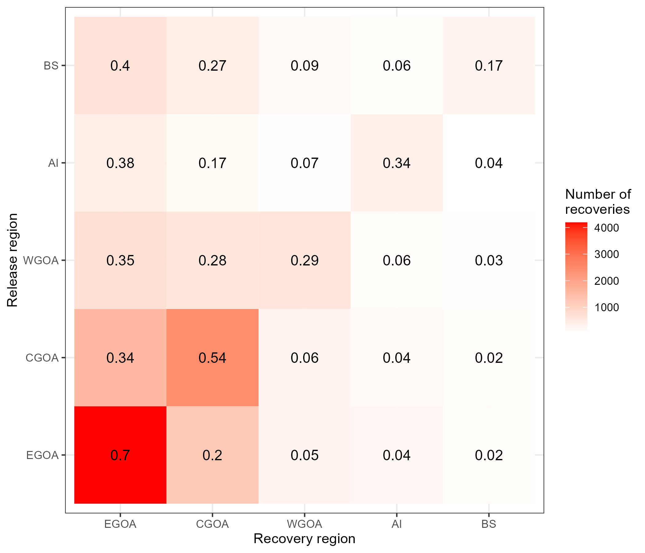
Figure 7.4: Tag recoveries by release and recovery region pooled over all years. Colors are number of tags recovered and text indicates the proportion.
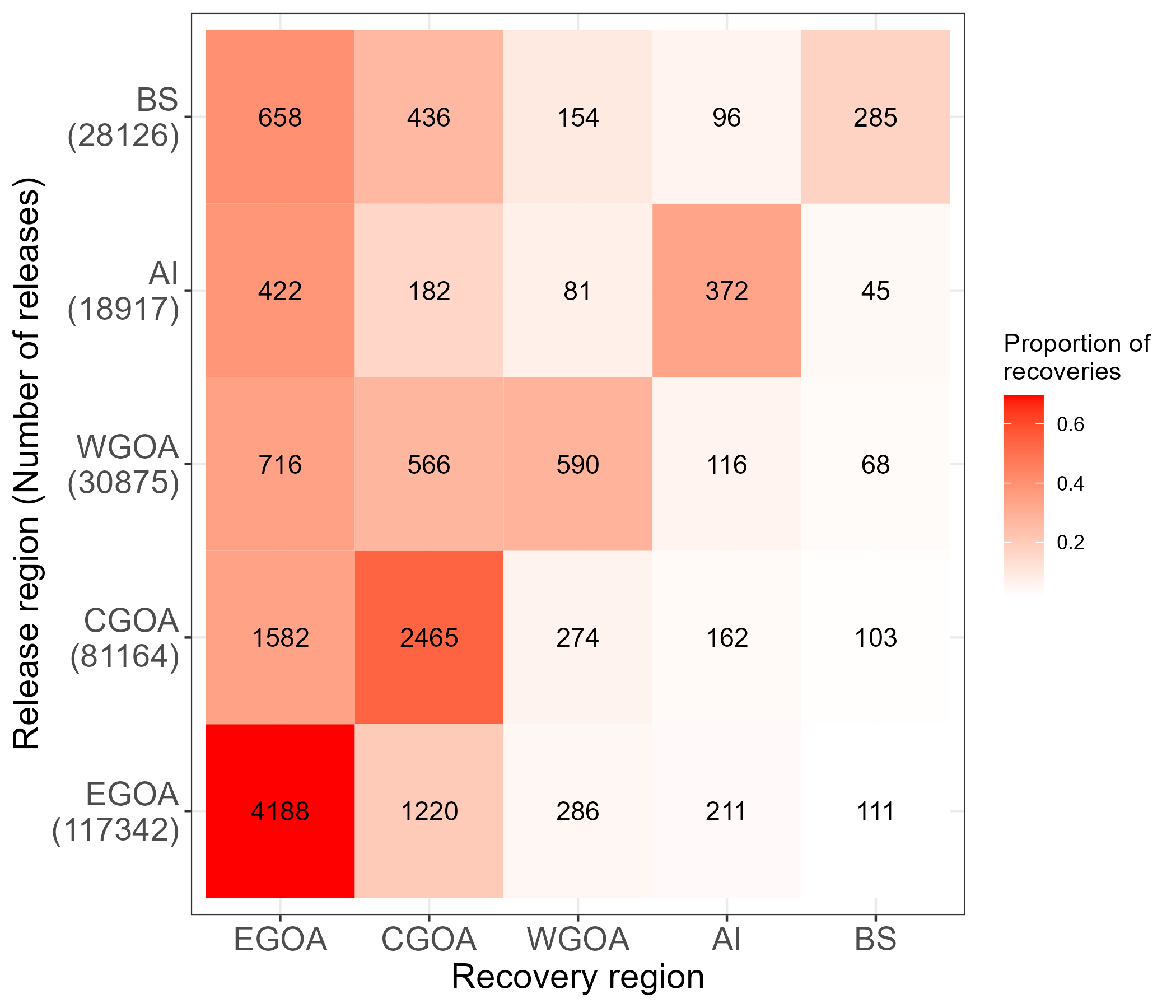
Figure 7.5: Tag recoveries by release and recovery region pooled over all years. Colors proportion of recoveries and text is the number of recoveries among recovery regions.
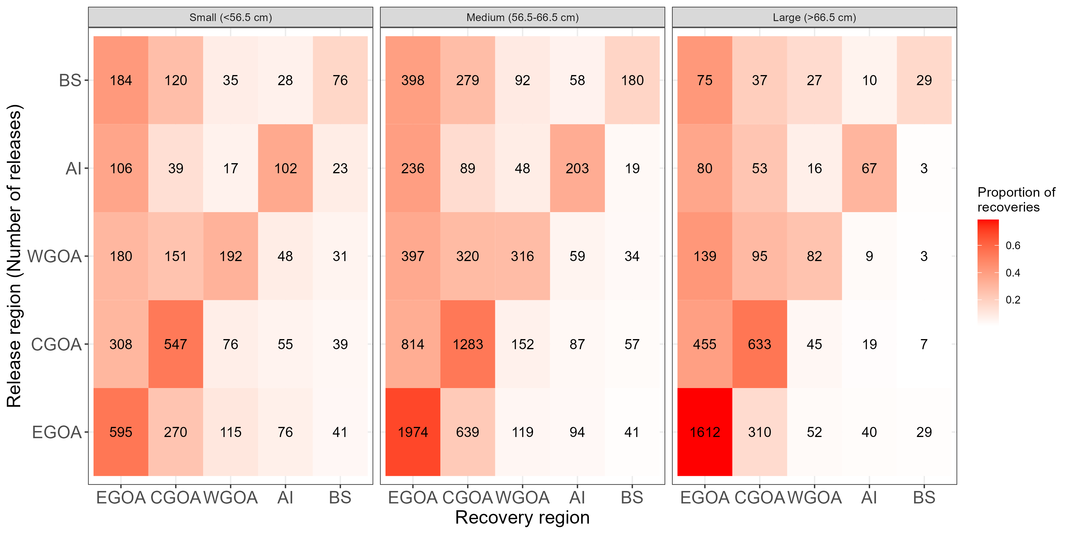
Figure 7.6: Tag recoveries by release and recovery region pooled over all years for different length groups. Colors are number of tags recovered and text indicates the proportion.
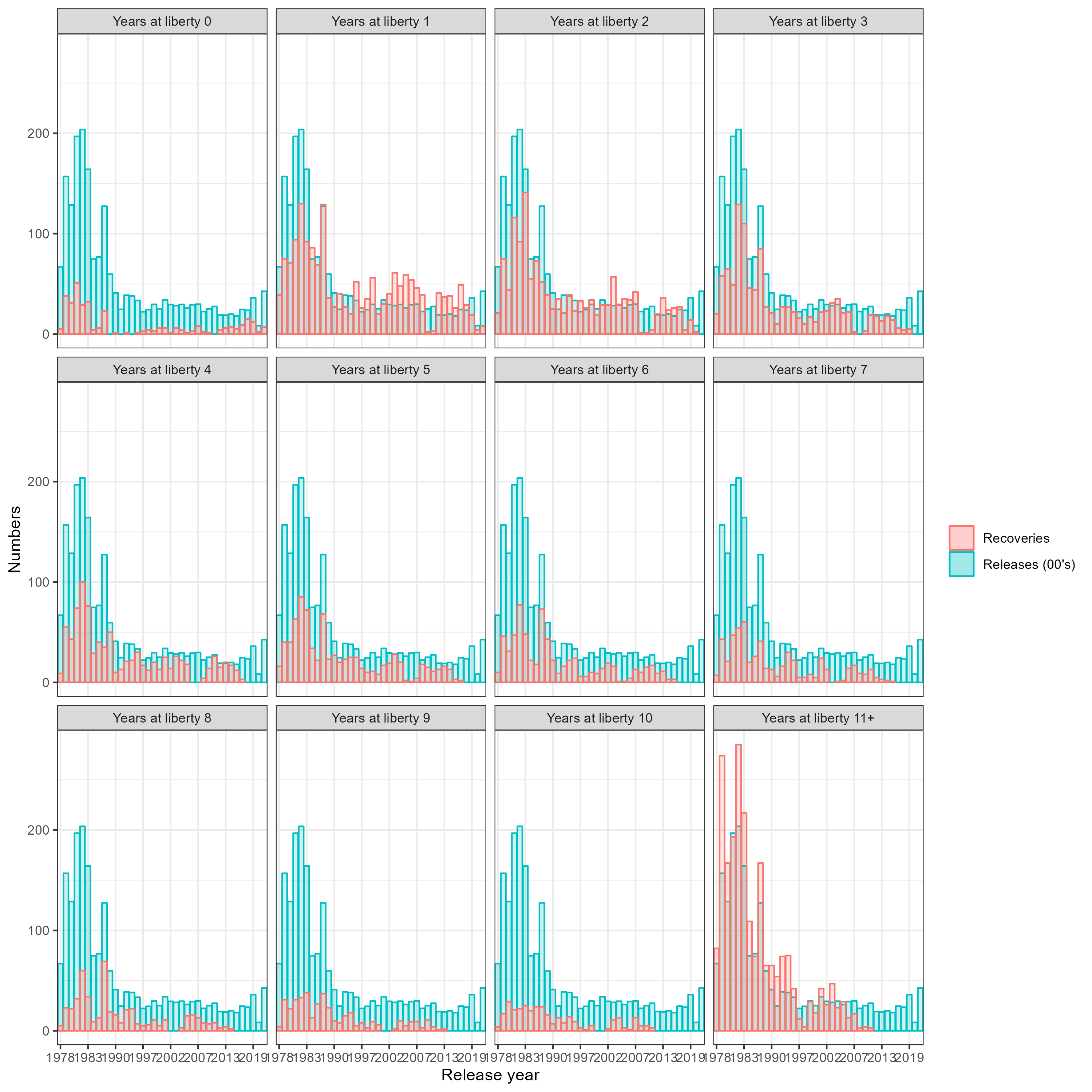
Figure 7.7: Number of tag recoveries and releases by release year and years at liberty
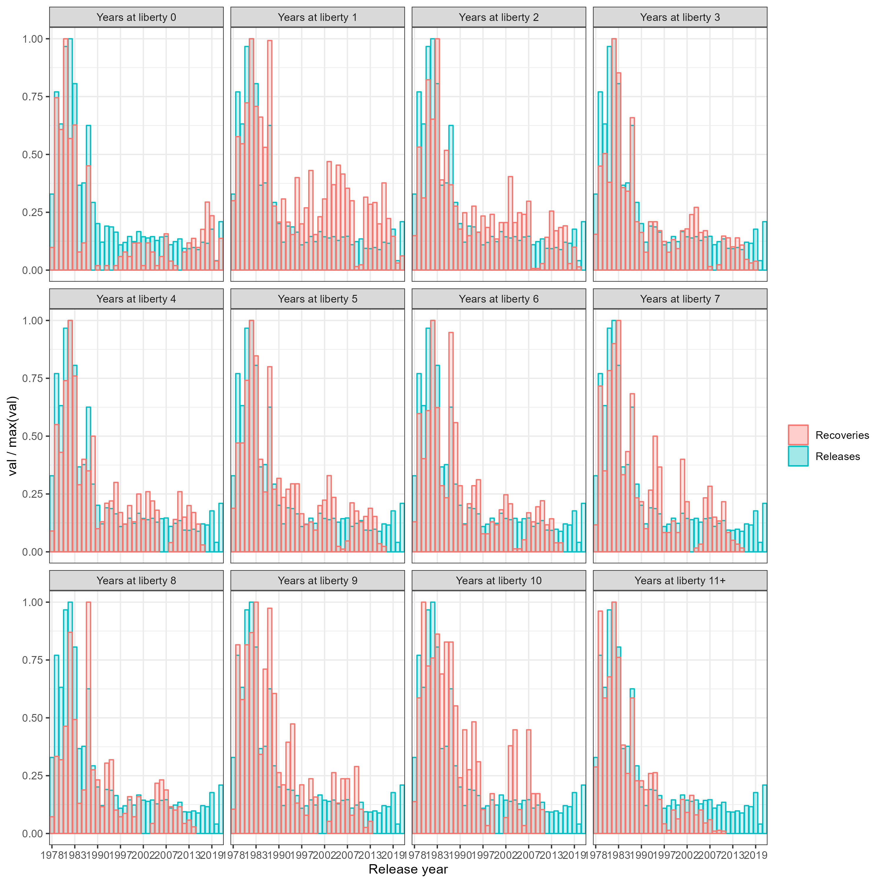
Figure 7.8: Relative (val/max(val)) tag recoveries and releases by release year and years at liberty
Single area recovery model
To get an idea regarding tag-mixing and expected recoveries we developed a simple recovery model that was loosely based on Fs and Ms assumed in the sablefish assessment. When we initially run the spatial model with the tagging data there was a scaling problem where the model wanted large annual fishing mortality rates. To explore this we focused on the single area model and looked at expected recoveries based on a range of tag-loss, annual tag-shedding and mortality assumptions
Three tag recovery models were explored
- \(\mathcal{M}_1\)
\[ \widehat{N}^{k}_y = \sum_a T^k_a \left(\exp{-Z_{a}}\right)^y \frac{F_{a}}{Z_{a}} (1 - e^{-Z_{a}})\]
- \(\mathcal{M}_2\)
\[ \widehat{N}^{k}_y = \sum_a T^k_a exp(-M_{tag}) \left(\exp{-Z_{a}}\right)^y \frac{F_{a}}{Z_{a}} (1 - e^{-Z_{a}})\]
- \(\mathcal{M}_2\)
\[ \widehat{N}^{k}_y = \sum_a T^k_a exp(-M_{tag}) \left( \exp{-(\tau + Z_{a})}\right)^y \frac{F_{a}}{Z_{a}} (1 - e^{-Z_{a}})\]
where, \(T^k_a\) numbers of tag releases, released in year \(k\) of age \(a\), \(y\) denotes years at liberty, \(F_{a} = 0.078 * S_a\), where \(S_a\) is logisitc selectivity with \(a_{50} = 5\) and \(ato_{95} = 2\) (the value 0.078 was the mean fishing mortality from the 2021 assessment), \(Z_a = F_a + 0.1\), \(M_{tag}\) is the initial tag induced mortality (=0.1), and \(\tau\) is the annual tag-shedding rate (=0.02). This ignores sex and assumes constant F over years, which is obviously incorrect. However, the purpose was to help identify release years that may be problematic due to mixing or perhaps higher tag induced mortality than initially assumed.
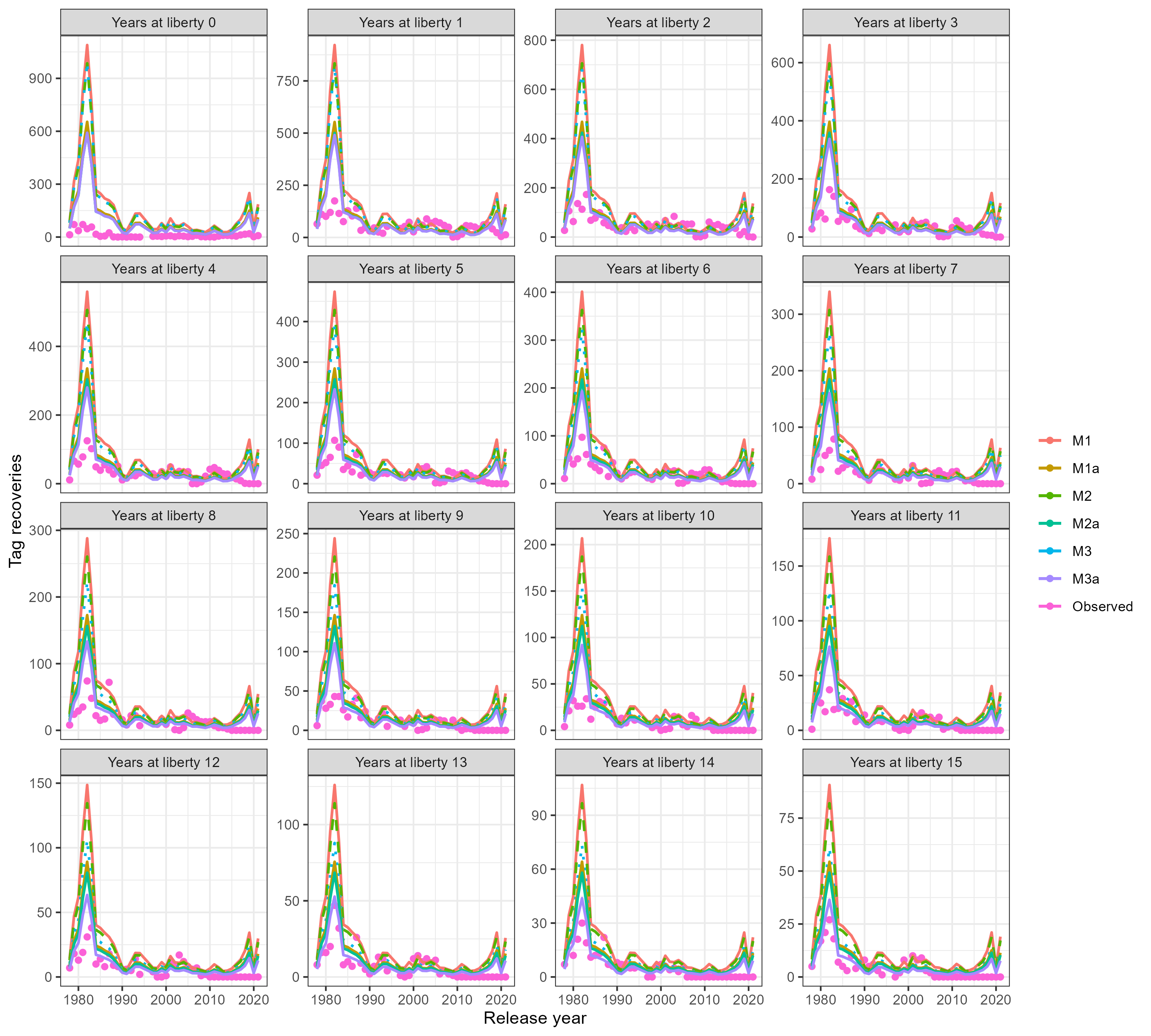
Figure 7.9: Observed and predicted recoveries from a simple model exploration. The a subscript in the model labels assumes tag-reporting of 60%, the absence of the subscript assume 100% tag reporting.
Lincoln-Peterson estimator
We applied a simple Lincoln-Peterson estimators to view changes in abundance over the area of interest using a subset of the tag recoveries. The Lincoln-Peterson estimator follows
\[ \widehat{N} = \frac{n e^{-(\kappa + M)}K\tau}{k} \ . \]
| Symbol | Description |
|---|---|
| \(N\) | Number of fish in the population |
| \(n\) | Number of fish released with a tag |
| \(K\) | Number of fish scanned for tags (fishery catch over the period of recoveries |
| \(k\) | Number of tagged fish recovered |
| \(\tau\) | Reporting/detection rate = 0.276 from Heifetz and Maloney (2001) |
| \(\kappa\) | Annual tag loss or mortality = 0.1 Beamish and McFarlane (1988) |
| \(M\) | Natural mortality = 0.1 based on D. Goethel et al. (2021) |
Most of the tags are released during the summer survey (Figure 7.10) but recoveries are more spread out within a year.
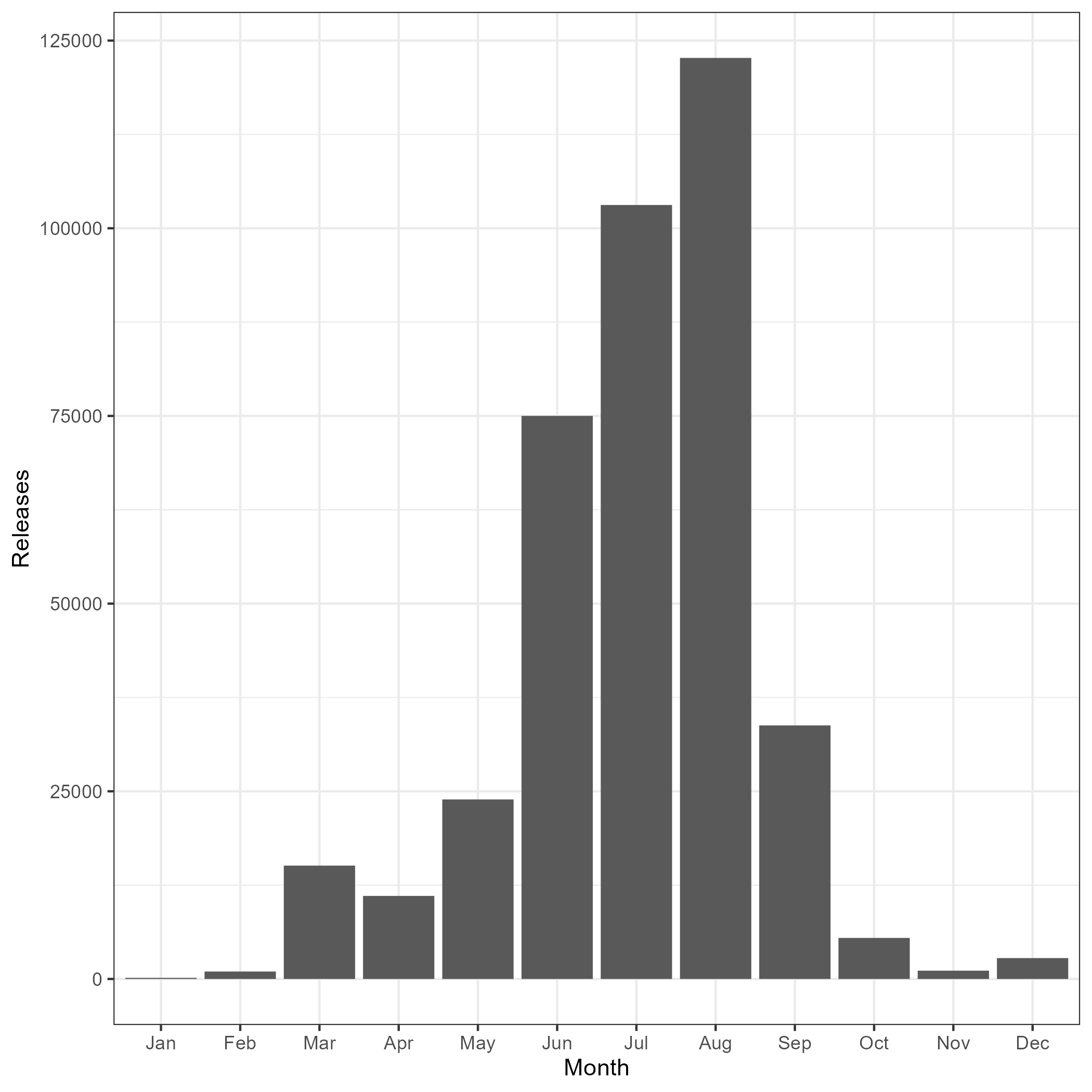
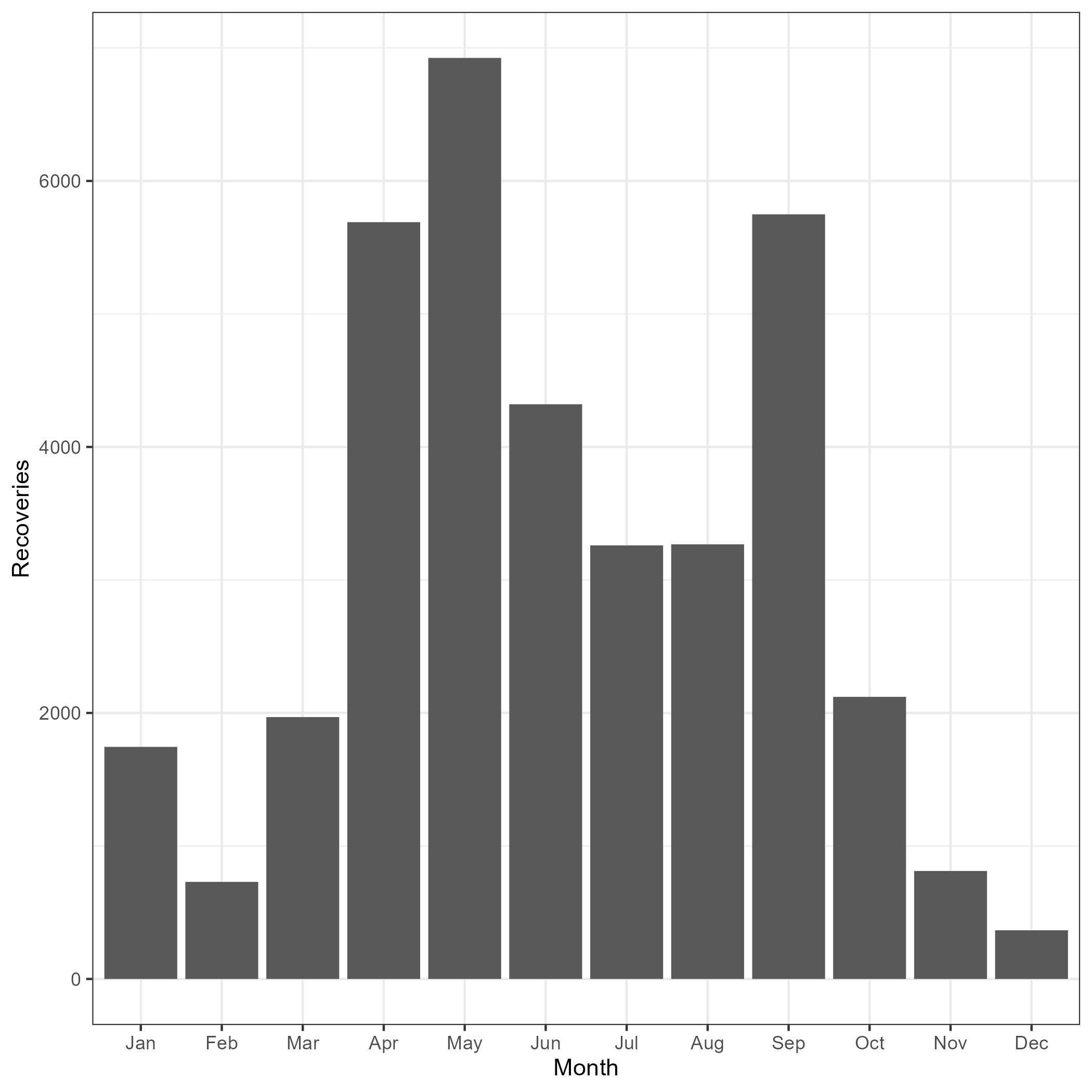
Figure 7.10: Tag recovery and release distributions by month
A Lincoln-Peterson estimator based on long line tag recoveries that were at liberty for a year (300 - 420 days) was explored. This time-at-liberty period was chosen so we could calculate annual estimates of abundance and thus derive annual estimates of exploitation rates to compare with the assessment. Due to the large distance traveled by sablefish over this time-period (Figure 7.11), the spatial extent considered was the entire stock region.
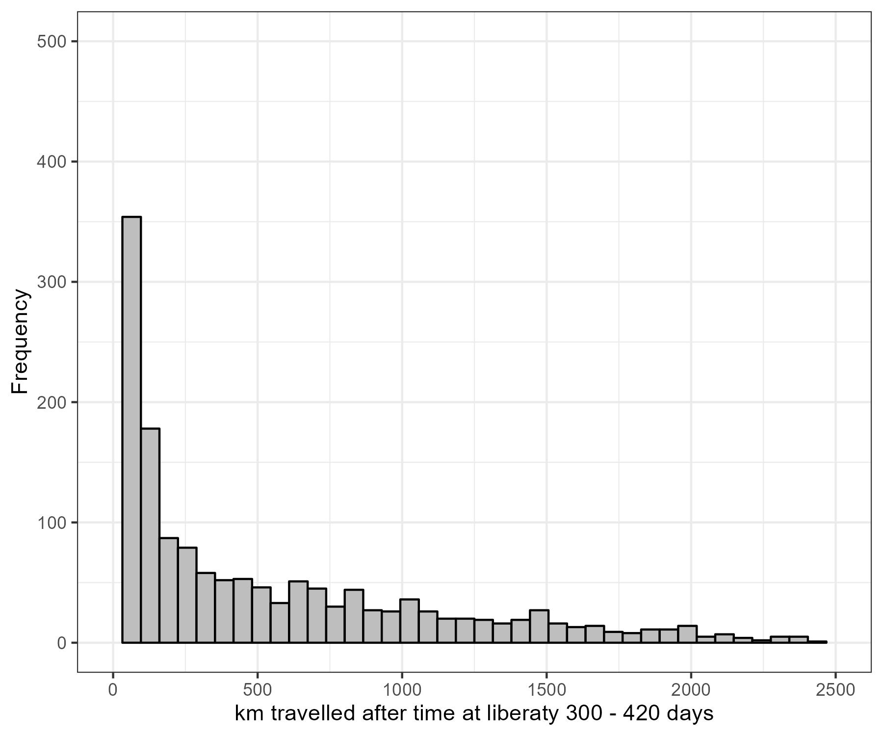
Figure 7.11: Distance (km) between release location and recovery location for fish at liberty for a year.
A few calculations/approximations are included in the Lincoln-Peterson estimator, these include tag loss and natural mortality for tagged fish after a year at liberaty, reporting rates from the commercial fishery, and changing reported weights to numbers. The period for calculating catch that was scanned during tag recoveries was the 15 of May to 15 of September. This was chosen as it brackets the monthly peak of releases (Figure 7.10). The other adjustment was converting reported weight into numbers. For this I calculated the mean numbers of fish per tonne based on the observer data. I then used this multiplier for the catch reported in tonnes during the period of recoveries to extract the numbers scanned by the fishery each year.
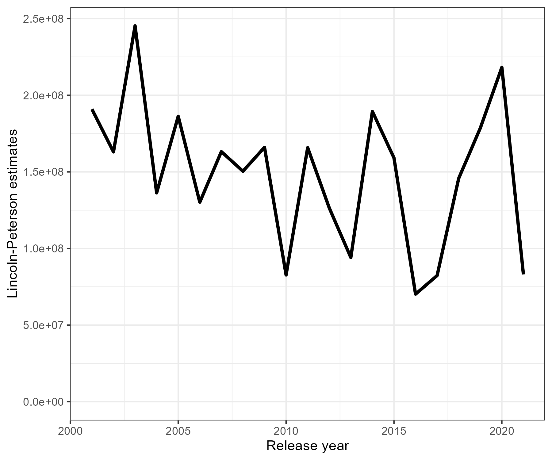
Figure 7.12: Recovered fish by gear type and year
Once we have annual population abundance estimates we can derive a rough annual exploitation rate (\(U_y\)) denoted by
\[ U_y = \frac{C_y}{\widehat{N}} \] where, \(C_y\) is the annual catch in numbers for the Longline fishery shown in Figure 7.13.
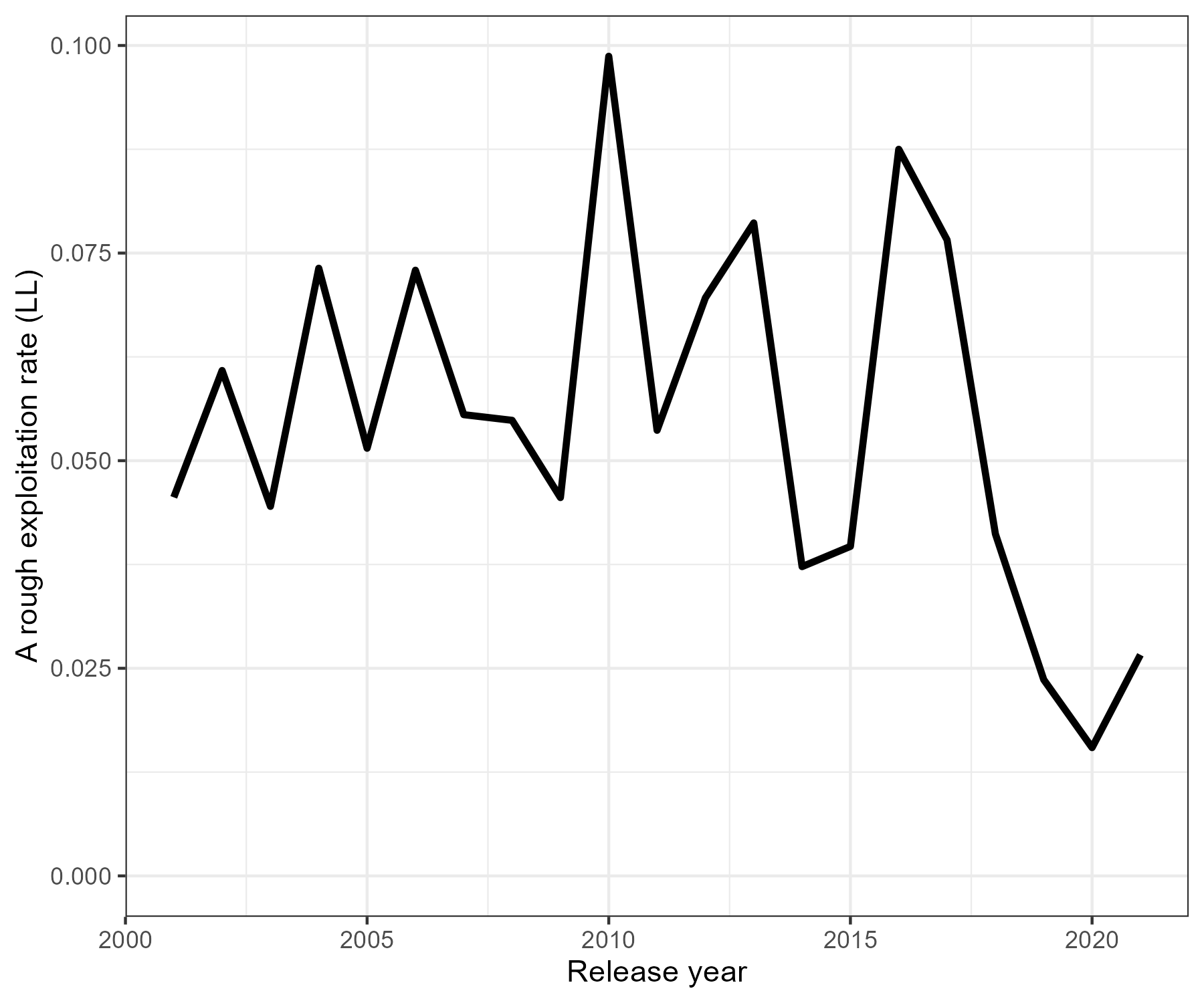
Figure 7.13: Exploitation rate for the Longline fishery based on Lincoln-Peterson estimates
Integrating tagging observations in spatial age-structured models
This project intends to explore a range of methods for utilizing tag-recovery observations in spatially disaggregated age-structured stock assessments.
Tagging things to consider with relevant references
- Years to retain tagged fish in the partition “After approximately 9 yr the number of recaptures was small and contributed more to the variance associated with the trends in movement than an improved understanding of these trends” Beamish and McFarlane (1988)
- Reporting rates (Heifetz and Maloney 2001)
- Scan detection rates. Is this not a factor of reporting rates?
- Mixing time and how to deal with it?
- Tag loss “tag loss in the fist year was approximately 10% and after that approximately 2% per year.” Beamish and McFarlane (1988)
- Release conditioning vs recapture conditioning (Vincent, Brenden, and Bence 2020; McGarvey and Feenstra 2002)
- likelihood choice? (Hanselman et al. 2015)
Releasing tags
Tag release events involve releasing a tag-cohort at the beginning of a year within a specific area. A tag cohort is indexed by \(k\) and has an implied year \(y\) and region \(r\) index. \(\boldsymbol{N}^k\) is used to denote a vector of lengths or ages for tag-cohort \(k\). In general, only the length frequency is known at time of release for each tag-cohort because ageing is a fatal process. We consider two different approaches for seeding a tag cohort within spatial age-structured models. The two methods are essentially the same but differ in whether the length are converted to age outside of the model (“External”) or done within the model (“Internal”). The internal method requires users to supply length frequency for each tag-cohort and the model will use the assumed growth assumptions and sex ratios to convert the lengths to ages. The external approach will use an age-length key outside of the model to derive an age frequency that can then be supplied to the model.
A frequent assumption of age-structured tagging models in the literature (Maunder 1998; Vincent, Brenden, and Bence 2020) is that the age-frequency of each tag-cohort is known. Due to the fact that ageing is a fatal process, we assume they have used the external approach. If the age-length key is representative, then this method is expected to be very similar and have better computational performance. Factors to consider at time of release are; gear method used to select releases, where releases occur, and time of releases. If growth is estimated within the assessment model, then the internal method may be prefered to keep the growth assumptions consistent between LF observations and other model quantities.
One down fall of the internal approach is tag releases and recoveries are both length-based inputs. Due to age-structured modelling growth as length conditional on age. Moving individuals back and forwards through the age-length transition matrix (length \(\rightarrow\) age \(\rightarrow\) length) will cause “smearing” of length frequencies. This is demonstrated in Figures @(ref:addagelength) and @(ref:showagelengthtransition_problem), and needs to be considered when considering model fitted values for observations and corresponding likelihood assumptions. Given this phenomenon, we make the argument that the external age-length key approach should be used. The external method means we assume (there actually is error in this) the ages of released fish and time at liberty, thus we know the age at recovery.
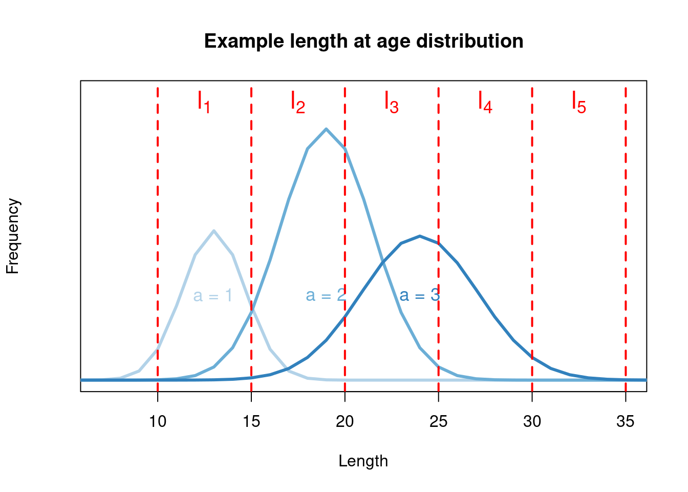
Figure 7.14: An example of theoretical length at age, with overlapping length bins used to describe the effect of going back and fourth through the age-length transition matrix.
## Warning: Using `size` aesthetic for lines was deprecated in ggplot2 3.4.0.
## ℹ Please use `linewidth` instead.
## This warning is displayed once every 8 hours.
## Call `lifecycle::last_lifecycle_warnings()` to see where this warning was
## generated.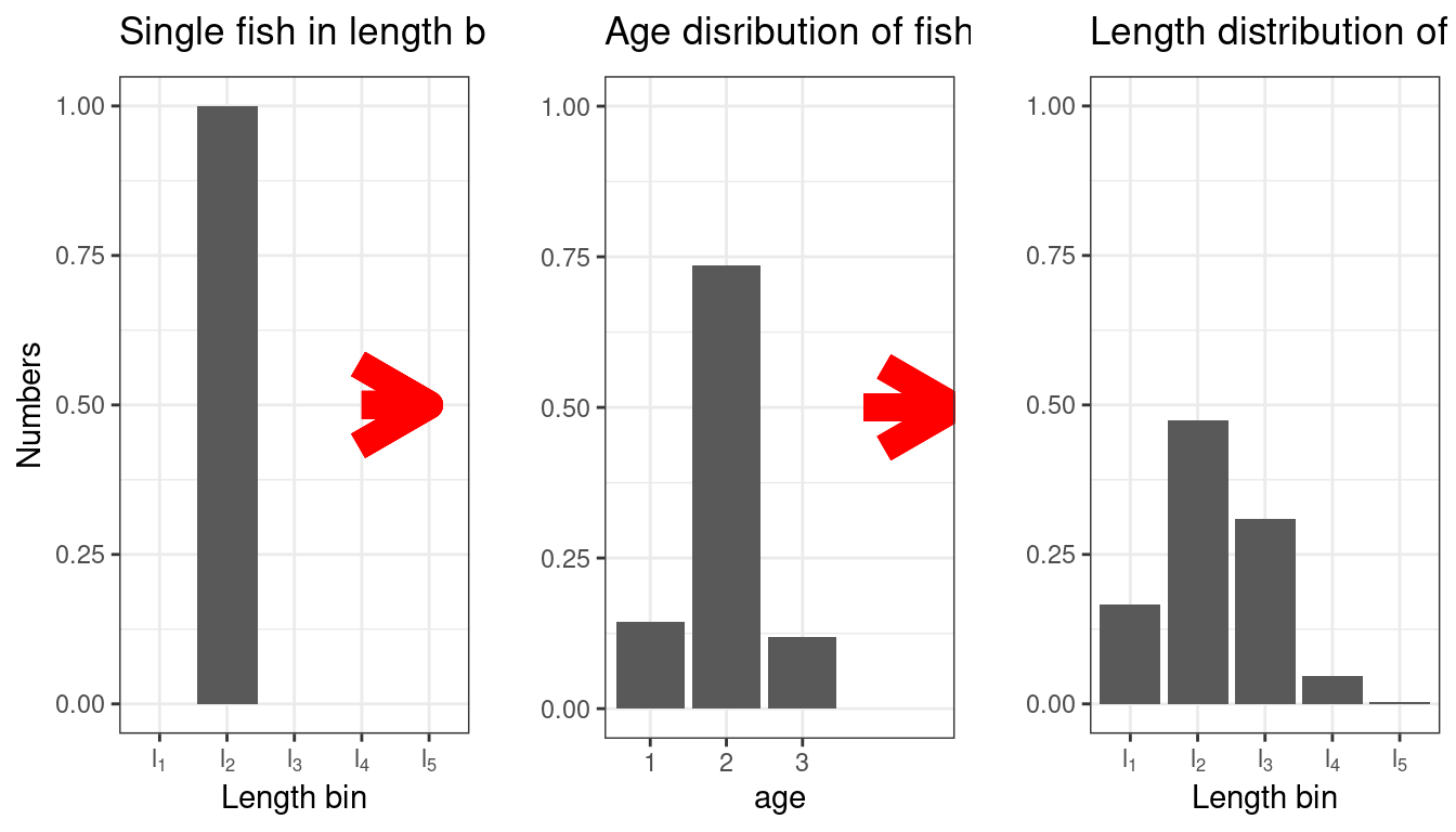
Figure 7.15: A visualisation of the effect of going back and forth through an age-length transition matrix. This can happen when tag releases and recaptures are input as length in an age-structured model. The model converts lengths to ages, then reconverts the age to length for observations. This is assuming the same age-length relationship in Figure 7.14
Internal method
Age-structured stock assessment models contain growth models, which describe length conditioned on age. This requires assumptions on the distribution and associated parameters. The default is often the normal distribution with mean length at age denoted by \(\bar{l}_a\) with standard deviation parameterised as a coefficient of variation (\(\sigma_a = cv*\mu_a\)). This information enables the model to derive a growth transition matrix \(P_{l|a}\). Given the lower and upper limits for each length bin denoted as \(\boldsymbol{b} = (b_1, b_2, \dots, b_{max})'\), the probability of being in length bin \(l\) given age \(a\)
\[\begin{equation} P_{l|a} = \begin{cases} \Phi(b_{l + 1}|\mu_a,\sigma_a)\quad &\text{for } l = 1\\ \Phi(b_{l + 1}|\mu_a,\sigma_a) - \Phi(b_l|\mu_a,\sigma_a)\quad &\text{for } 1 < l < n_l\\ 1 - \Phi(b_{l}|\mu_a,\sigma_a)\quad &\text{for } l = n_l \end{cases} \tag{3.6} \end{equation}\]
where \(\Phi(x|\mu,\sigma)\) is the cumulative normal (but could be generalised to any probability distribution). If growth varies by attributes such as sex, stock or region then this will need to be calculated for each growth model.
At the point a tag cohort is released, the model can derive the length composition of the vulnerable population using the transition matrix derived in Equation (eq:agelengthtransition). Given the number of estimable parameters that govern the age-stricture at a point in time and growth model, an exploitation rate is calculated so that if there are not enough numbers in a length bin to be tagged, a penalty can be added to the objective function to dissuade the combination of parameters that generated this situation. Tag-release by length is a known quantity and so the model must allow for a minimum vulnerable length composition to that released. To enforce this, an exploitation rate by length \((u_l)\) is calculated as follows, \[\begin{equation} u_l = \frac{N^k_{l}}{\sum_a}N_{y_k,a,r_k} P_{l|a} \tag{7.1} \end{equation}\]
During parameter estimation there are no constraints within the model to trial a set of parameters that will allow \(u_l > 1\) i.e., more observed tag-releases than in the available population. To stop negative numbers at age, \(u_l\) is set at a level less than 1 and a penalty added to the objective function to discourage parameters from allowing this condition. Finally, tag-release at age is calculated as follows, \[\begin{equation} N^k_{a} = N_{y_k,a,r_k} P_{l|a} u_l \tag{7.2} \end{equation}\]
Once the tag cohort are created in the model it is assumed that tagged fish are exposed to the same dynamics as un-tagged fish. Revisit this we will want to explore mixing behaviour/assumptions.
External method (Age-length key method)
Once a tag-release event has occurred for tag group \(k\), the only known knowledge is the length distribution \(N^k_l\). Assuming there is an accessible forward age-length key which describes the proportion of ages for a given length bin \(\left(P_{a|l}\right)\) that is representative of the vulnerable population to tagging for the same area and time, then the “forward” or “classic” key method can be used Ailloud and Hoenig (2019). If tag-release coincide with a fishing season you could use fishery-dependent derived age length information, assuming the selectivity curves within a length bin are parallel. If only a subset of fish from each haul are released, it would be better to construct an age-length key from a representative sample of fish that were caught but not-tagged. This would be relevant for single vessel survey release events. \[\begin{equation} N^k_a = \sum\limits_{l = 1}P_{a|l}N^k_l \end{equation}\] where, \(N^k_a\) is used as an known input into the model with no error. Revist can we account for uncertainty here?