Chapter 8 Initial model setup
Use Punt (2019) to outline the key considerations
- When did we choose to start the model and why. was it assumed to be in an equilibrium state
- What spatial regions did we start with and why
- How many fisheries?
- What observations were included? how were they initially weighted
Model start time
The start year for the current stock assessment is 1960. This is the earliest year in which catch is available. There is early sex-aggregated length composition from the Japanese longline fleet along with a CPUE index for that same fleet in the 60’s/70’s. The survey data doesn’t kick in until mid to late 70’s. Unfortunately catch is the most limiting data input, where we can only go back to 1977 before we loose information on regional catch be gear method (pers comms kari Fenske). For this reason 1977 was the start year for the spatial assessment model.
Model spatial resolution of the model
This section describes the decision making process we took in configuring an initial spatial model. The first consideration was whether to include areas outside of the Gulf of Alaska (GOA) and the Bering sea Aleutian islands region, which is the spatial extent for the current stock assessment (D. Goethel et al. 2021). Sablefish inhabit a broad spatial distribution from the northeastern Pacific Ocean from northern Mexico to the Gulf of Alaska. It is currently assessed by three assessment bodies, the first is the area of focus, being the Bering sea and gulf of Alaska (D. Goethel et al. 2021), one off the west coast of Canada (Cox et al. 2011) and the west coast from California to Oregon (Stewart et al. 2011). Given the complex juvenile life history coupled with long range movement capabilities of adults, the stock structure of sablefish has been a topic of extensive research.
A recent genetic study by Jasonowicz et al. (2017), found no significant difference between samples off the west coast of US, GOA and Bering sea (there were no samples off the west coast of Canada in this study), providing evidence for a single panmictic population. A recent morphometric study (M. Kapur et al. 2020), found significant differences in fish traits such as length at age between samples from the west coast of US and GOA. These results were consistent with the findings from Tripp-Valdez et al. (2012). Tagging is another important information source, with extensive tag releases along the entire North Pacific. Tag recovery data provide evidence for a two stock hypothesis (Kimura and Shavy 1998). With a stock north of Vancouver Island and a stock to the south.
For the purposes of this research, we will assume GOA and BS, hereinafter refereed to as the GOABS complex, is isolated (i.e., no movement in or out of this region) from Canada and the west coast of the US. Although there is evidence to include part of Canada (Figure 7.3). Due to practical considerations regarding data sharing and the time-frame of this research Canada was excluded. The focus of this research is to build and explore a spatially explicit model for the GOABS complex.
The general approach taken, was to build an initial spatial model that had the finest spatial resolution possible and aggregate regions as data limitations and model convergence issues arose. This finest model spatial resolution was initially based on the input data set with the coarsest reported spatial resolution. Data sets have been reported at different spatial resolutions over time. In general, data are reproted at three levels of spatial resolution: latitude and longitude (high spatial resolution), statistical area (Figure 8.1) and larger fishery management boundaries (Figure 8.2). Input data sets and the spatial resolution available are described in the following table.
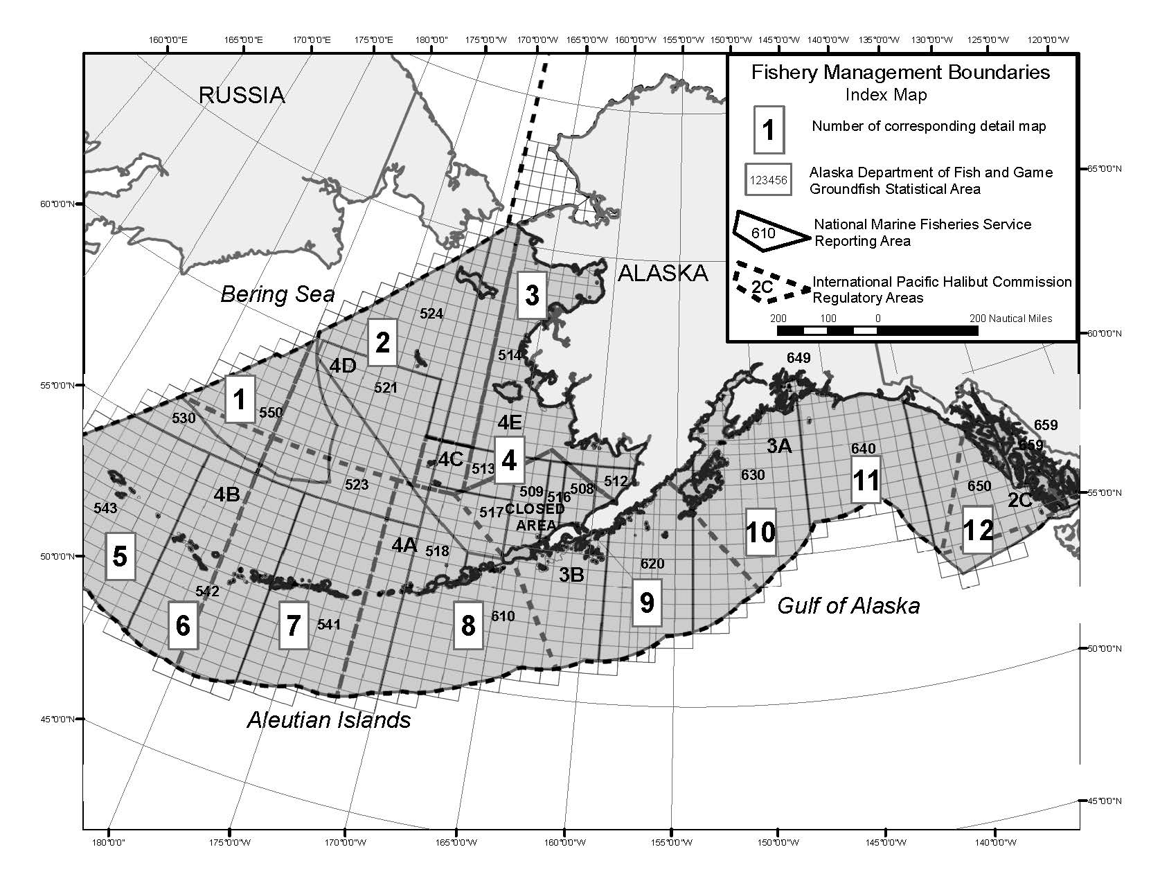
Figure 8.1: Statistical and reporting areas for GOABS complex
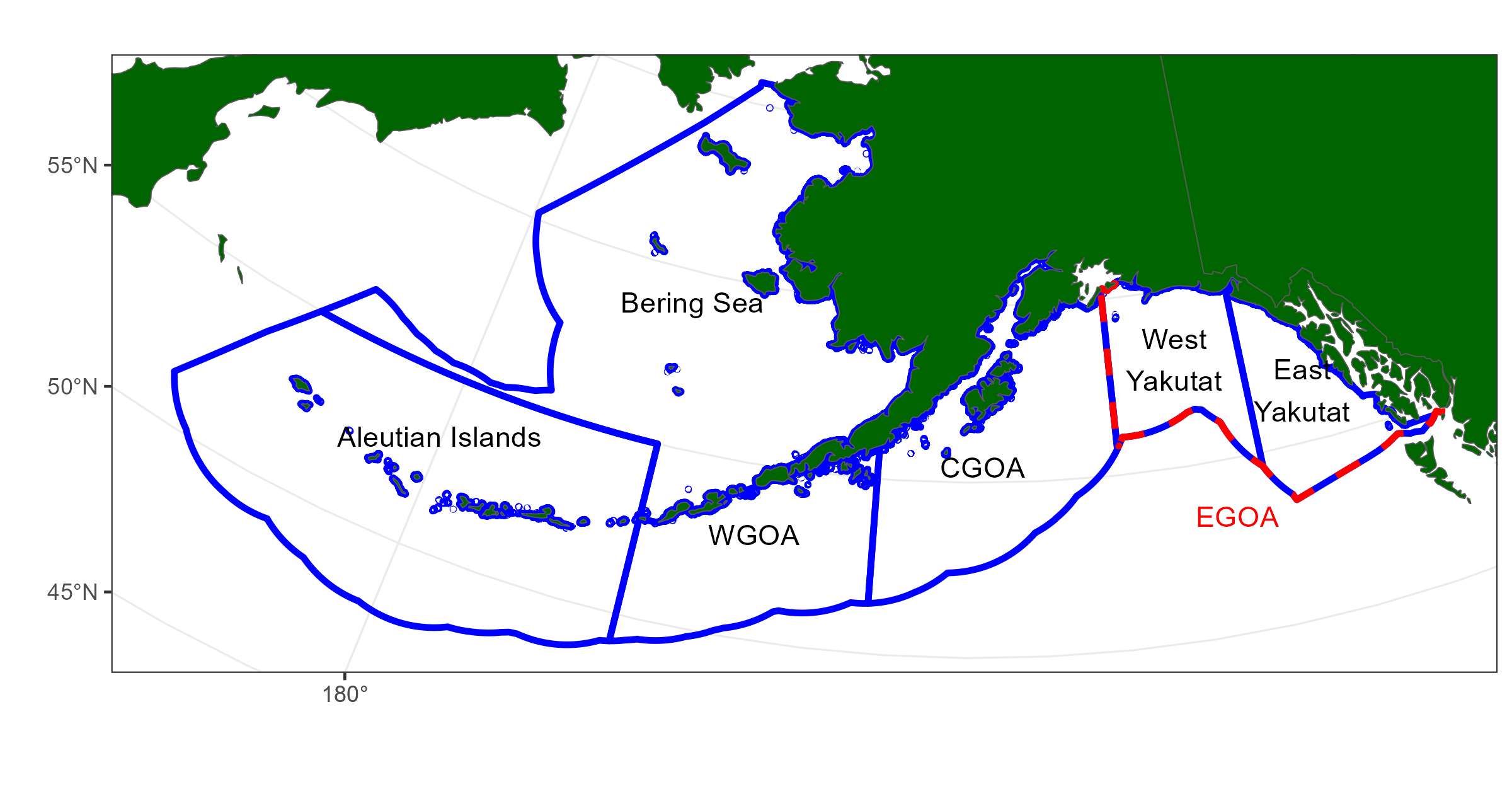
Figure 8.2: Fishery management plan boundaries. The Eastern Gulf is often reported at subareas split up be East/West Yakutat and sometimes Southeast.
| Data source | Description and spatial resolution |
|---|---|
| Catch pre 1990 | Available at FMP spatial resolution |
| Catch post 1990 | Available at FMP spatial resolution |
| Observer data (Age,Length and catch) | Latitude and Longitude positions |
| Survey data (Age, Length and catch) | Latitude and Longitude positions |
| Tagging data | Latitude and Longitude for releases, Latitude and longitude for approximately half the recoveries |
Reported catch from commercial fishers seems to be the most limiting data set which has the coarsest reported spatial resolution (check this statement). For this reason, the finest spatial resolution we will consider is the fishery management plan boundaries (FMP) being, Bering Sea, Aleutian Islands, Western Gulf, Central Gulf and Eastern Gulf i.e., five area model (Figure 8.3). Although this was determined by a reporting constraint, this is also the spatial resolution that ABC’s are allocated for
In addition to the reported spatial resolution of the data, we need to consider if there is any spatial sampling stratification within a data set. Sampling designs that have spatially varying stratification and thus spatially varying sampling intensity, could be inappropriate to use for alternative spatial stratifications. Often post-stratified estimators are not as efficient or accurate as design based estimators that are consistent with the sampling design. Fortunately in this case, the independent survey design is systematic. This results in consistent spatial sampling with respect to space, and removes this concern when considering alternative regional boundaries.
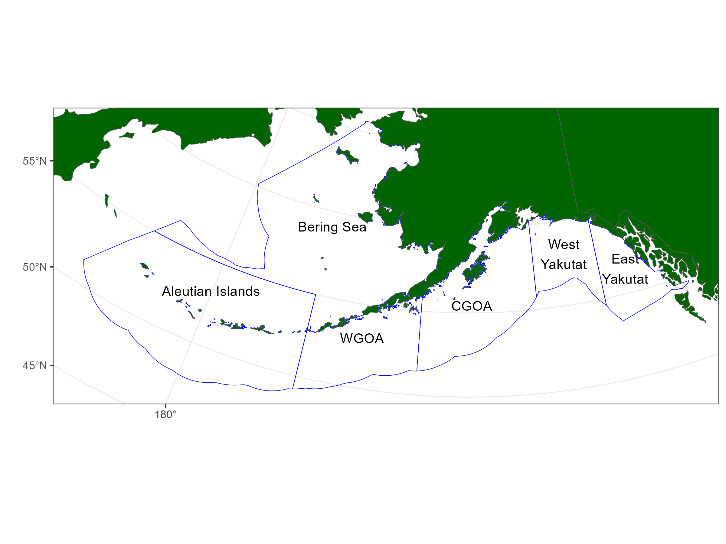
Figure 8.3: The finest spatial resolution that we are considering for Sablefish assessment
Fishery structure
I used the approach from Lennert-Cody et al. (2010) to analysis length frequency samples to identify changes in length frequency that may suggest alternative fleet or stock structures. My understanding of the method described in Lennert-Cody et al. (2010) is that it uses regression trees to identify splits/nodes in the covariates latitude, longitude and season that generate groups/clusters of length frequency distributions that are similar or somewhat homogenous. “Assuming sampling coverage is adequate, comparison of pooled and individual-year tree results can identify spatial structure that is strongly indicated in every year, and that which is only present in select years, perhaps as a result of strong recruitment or changes in catchability, or if sampling coverage is not adequate, sampling variability.”
A limitation for this method for our application is latitude and longitude grids contain unequal areas due to the shrinking of longitudes towards the poles. Also with the unusual shape of the coastline binary splits by latitude and longitude may also be a problem.
| Variable | Split value | Cell | Variance explained (%) | |
|---|---|---|---|---|
| Split1 | Lon | 180 | NA | 6 |
| Split2 | Year | 2015 | 2 | 10 |
| Split3 | Lon | 212 | 2 | 13 |
| Split4 | Lon | 206 | 4 | 14 |
| Split5 | Qrt | 12;34 | 2 | 15 |
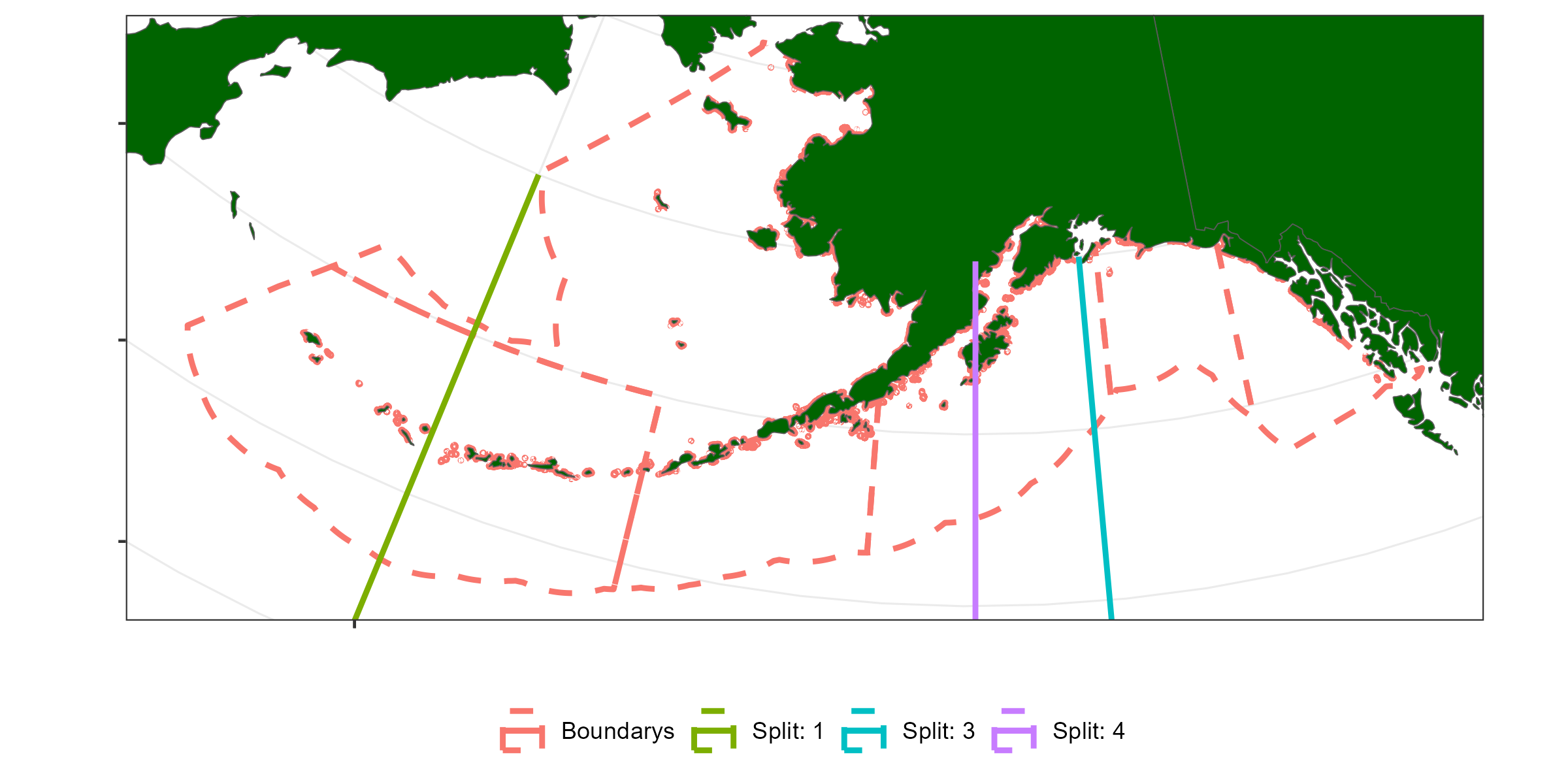
Figure 8.4: Longitude splits based on regression tree analysis from Table 8.1
A summary of fishing effort distributions by region and year. This plots the depth latitude and longitude within one of the five regions for observed fishing events.
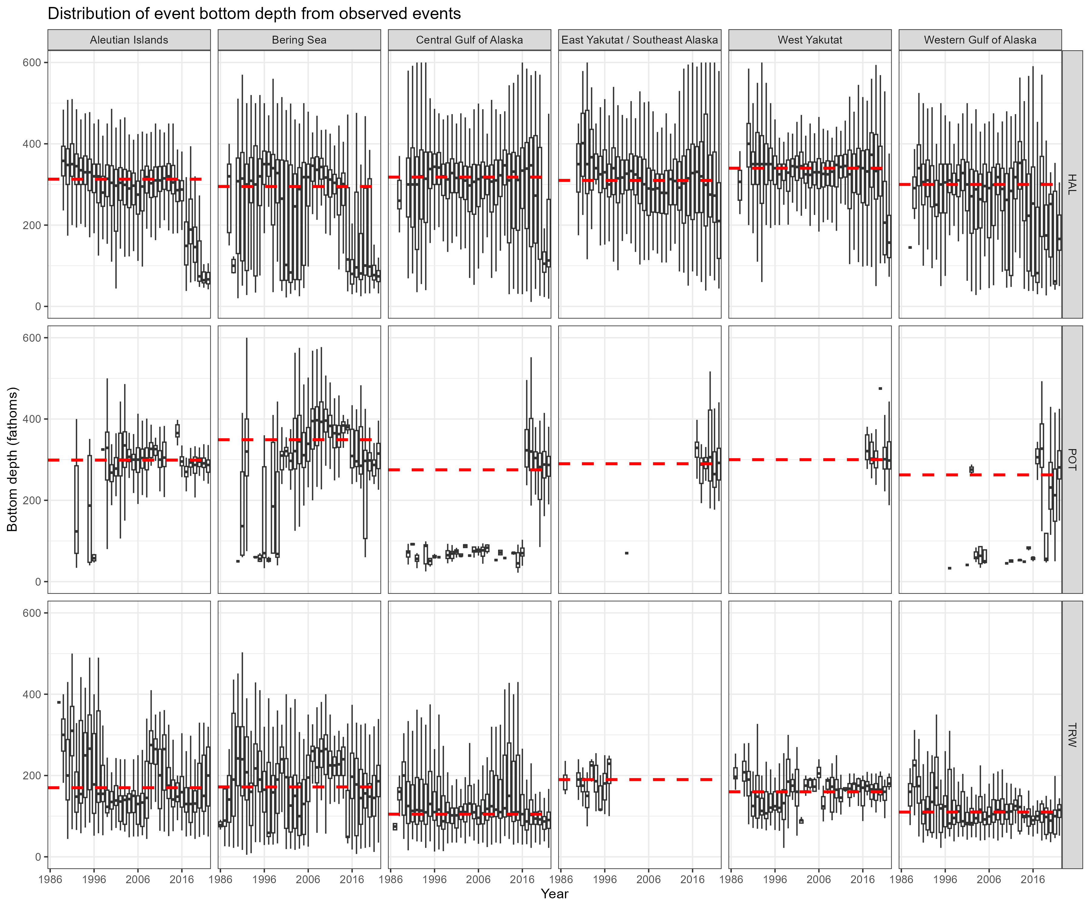
Figure 8.5: Boxplot of depth by observed fishing event
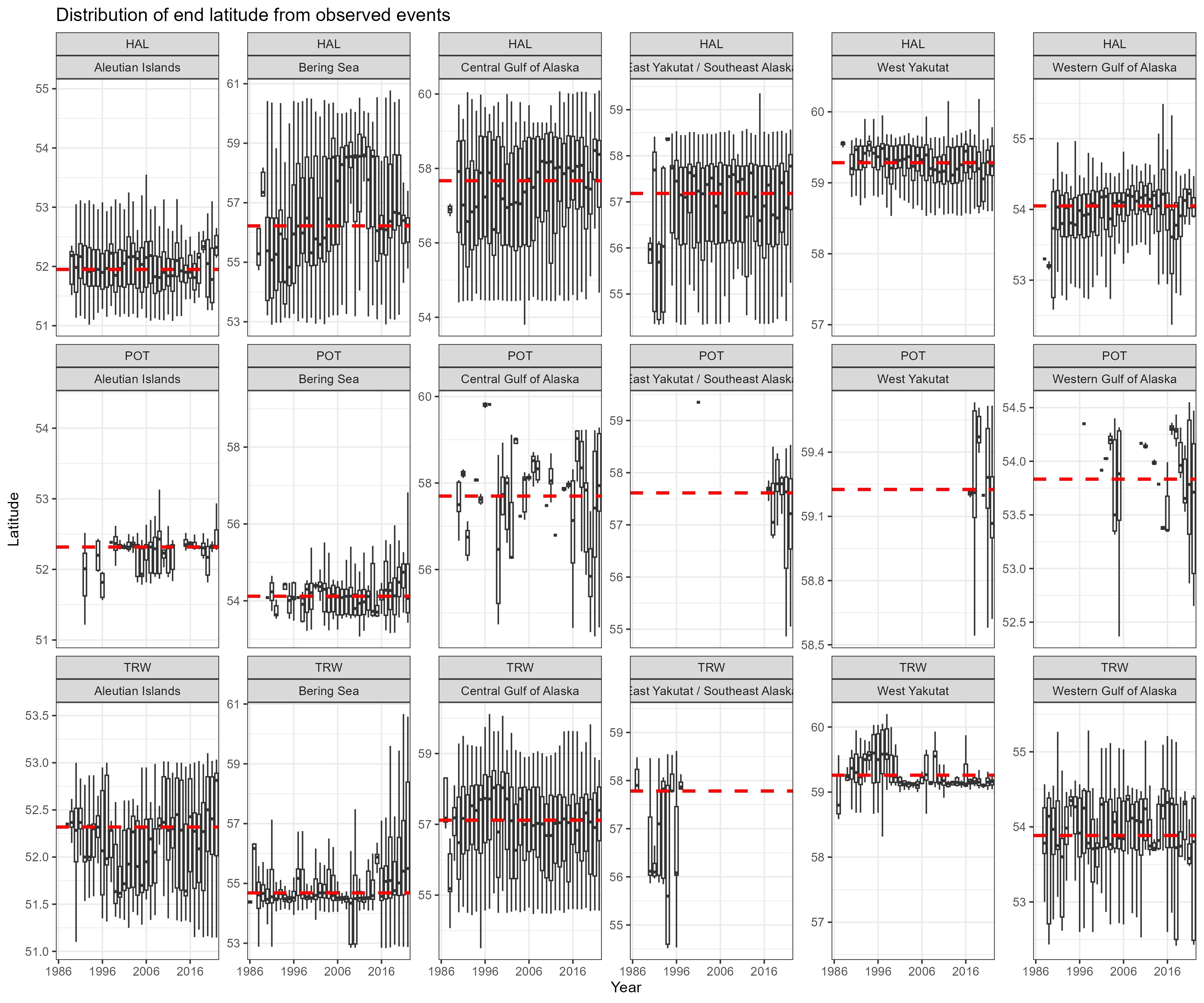
Figure 8.6: Boxplot of latitude by observed fishing event
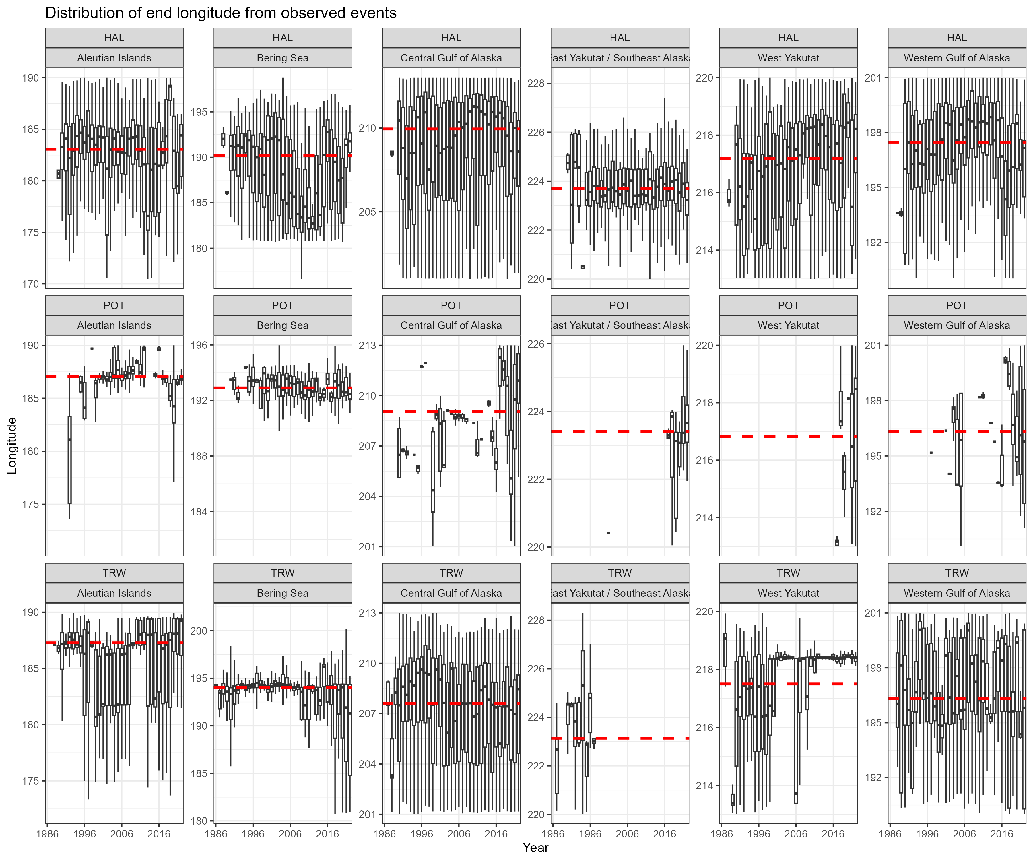
Figure 8.7: Boxplot of longitude by observed fishing event
Repeat regression analysis on survey LF data
I repeated the regression tree analysis for LF data on the survey data to see what spatial and temporal structures are in the Survey LF data. Interestingly it chose to have a longitude split at 206 degrees which was present in the fixed gear LF analsyis and the same break out at the Aleutian islands.
| Variable | Split value | Cell | Variance explained (%) | |
|---|---|---|---|---|
| Split1 | Year | 2015 | NA | 13 |
| Split2 | Lon | 206 | 1 | 19 |
| Split3 | Lon | 178 | 1 | 23 |
| Split4 | Year | 1986 | 3 | 25 |
| Split5 | Lon | 206 | 5 | 28 |
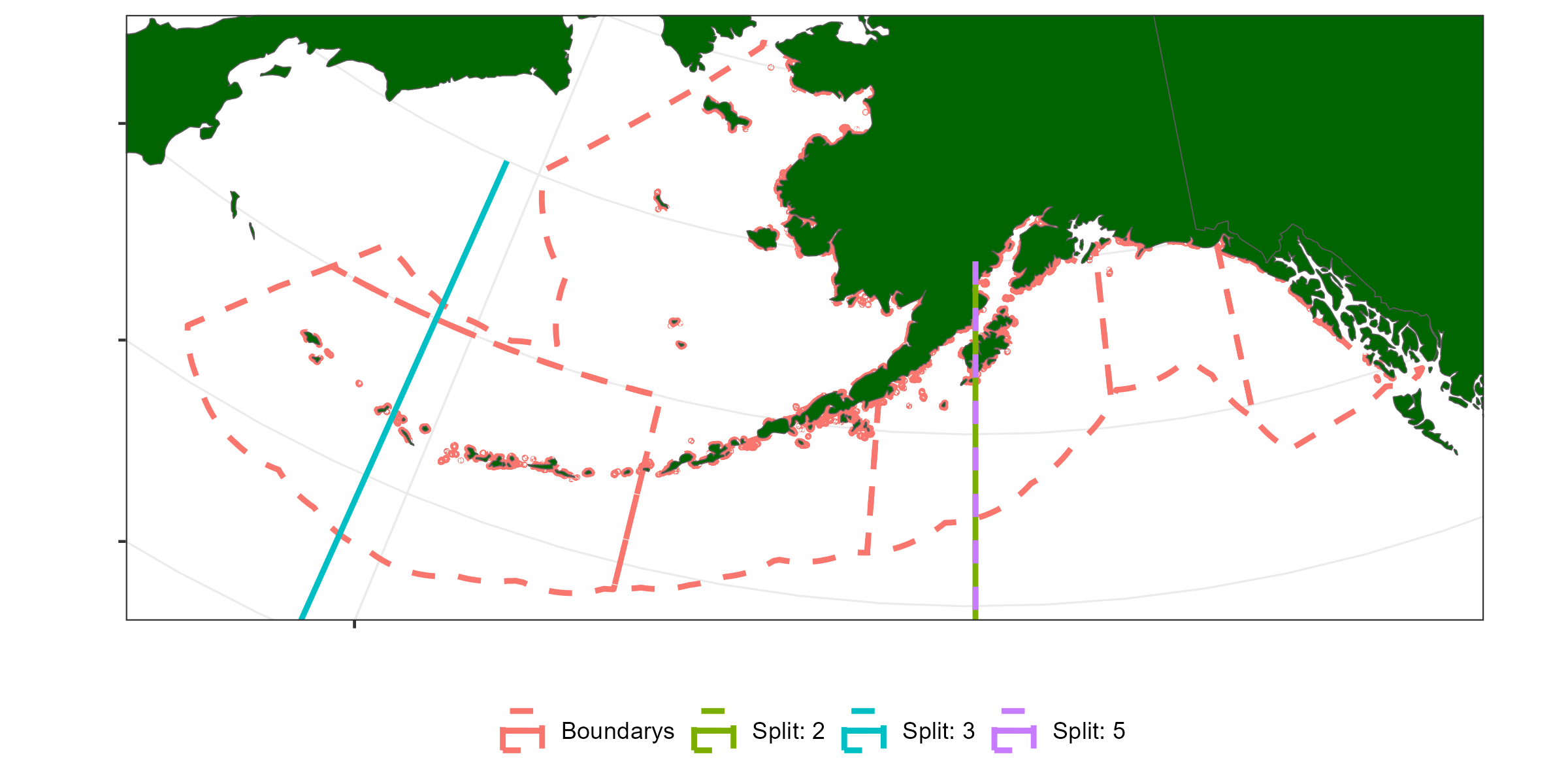
Figure 8.8: Longitude splits based on regression tree analysis from Table 8.2