Chapter 6 Fishery dependent data
This chapter describes an exploratory analysis using the observer and other fishery reported data. The aim is to highlight trends and signals in the data that would lead to an assessment decision or consideration e.g. spatial and temporal structures. All data analysed in this section has been extracted from the AKFIN database (North Pacific Observer Program). It included extracts from the length, age and catch reports. Some of the data cannot be displayed here due to confidentiality reasons. Locations shown in this work have been generalized to generic center locations of a 20 x 20 sq. km grid if there were 3 or more unique vessels, as per NOAA/NMFS regulations.
This data will result in two important assessment inputs: observed catch (which will be assumed known with a high level of precision) and composition by fishery, either age or length.
Define what a fishery is? Currently a “fishery” is defined by a gear type i.e., trawl vs fixed-gear (line and pot).
is there evidence for changing selectivity? i.e., time-blocks
Auxiliary information see Table 3.3 D. Goethel et al. (2021) for management actions which describe spatial closures by gear.
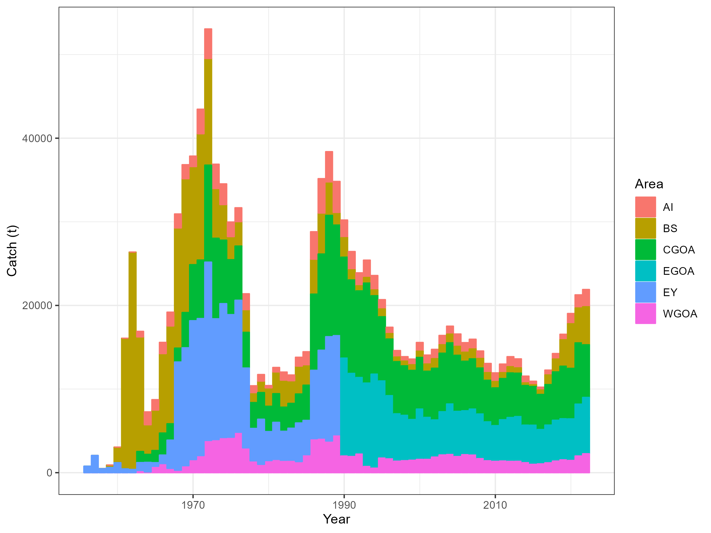
Figure 6.1: Catch history by region
Catch data
Deriving annual estimates of catch by year and region should be fairly straight forward. Fishers generally have a legal requirement to record catches and we will probably just assume that reported catches are accurate. Unfortunately catch by gear type and region is not known prior to 1977 (pers comms Kari Fenske).
The following bubble plots display the proportion of catch sampled for lengths and ages by observers relative to the catch by gear and area from 1990 when observer data available. When bubbles and crosses have the same size then the observer samples are proportional to catch for a given year. When crosses are larger then observers sampled more relative to the catch and vice versa. These are meant to give some impression of “representative” sampling i.e., are there regions or gears that are under or over sampled.
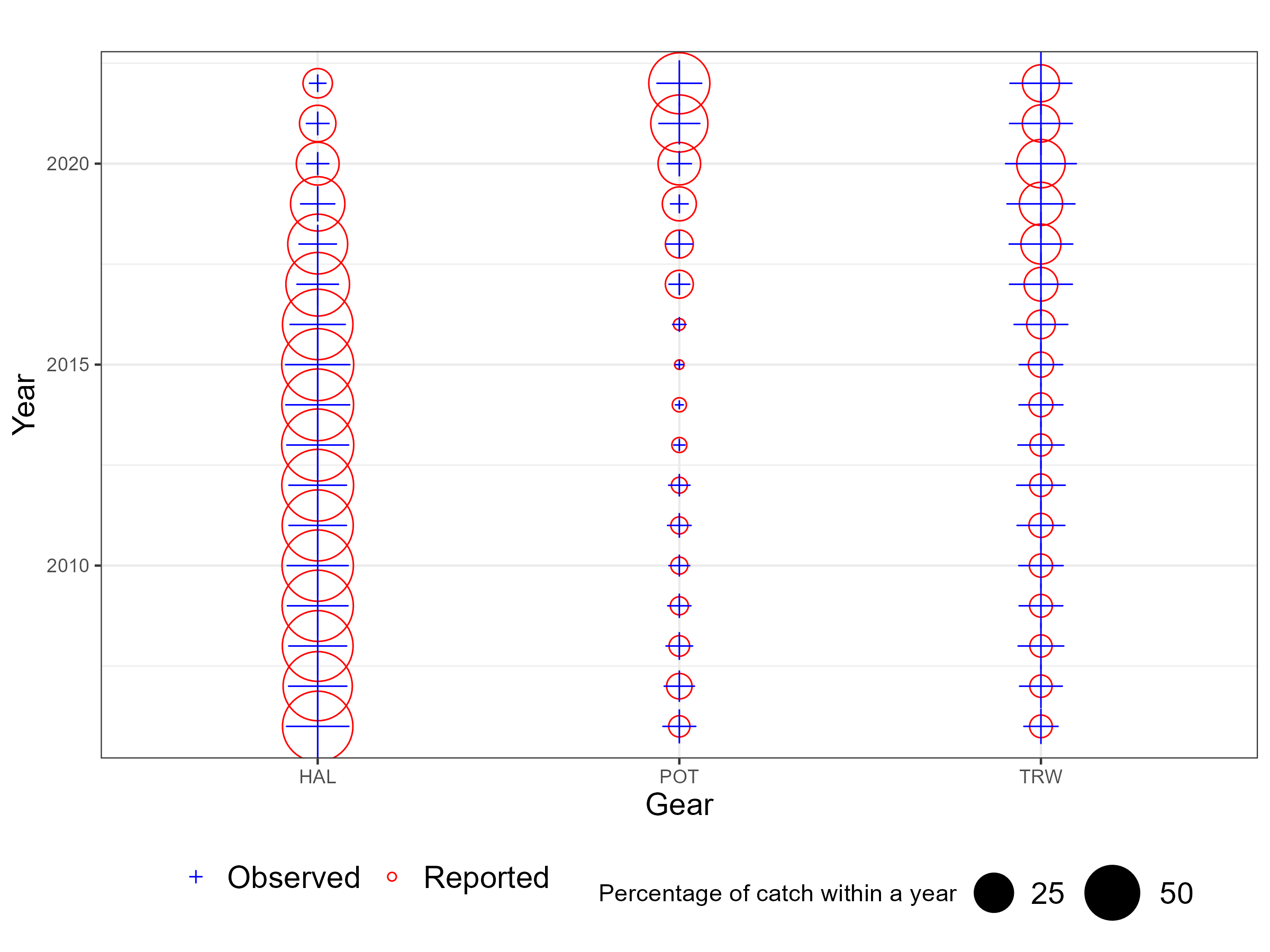
Figure 6.2: Observer representative figures by method. When the cross and circle are the same size this indicates observers sample proportional to the catch for a year.
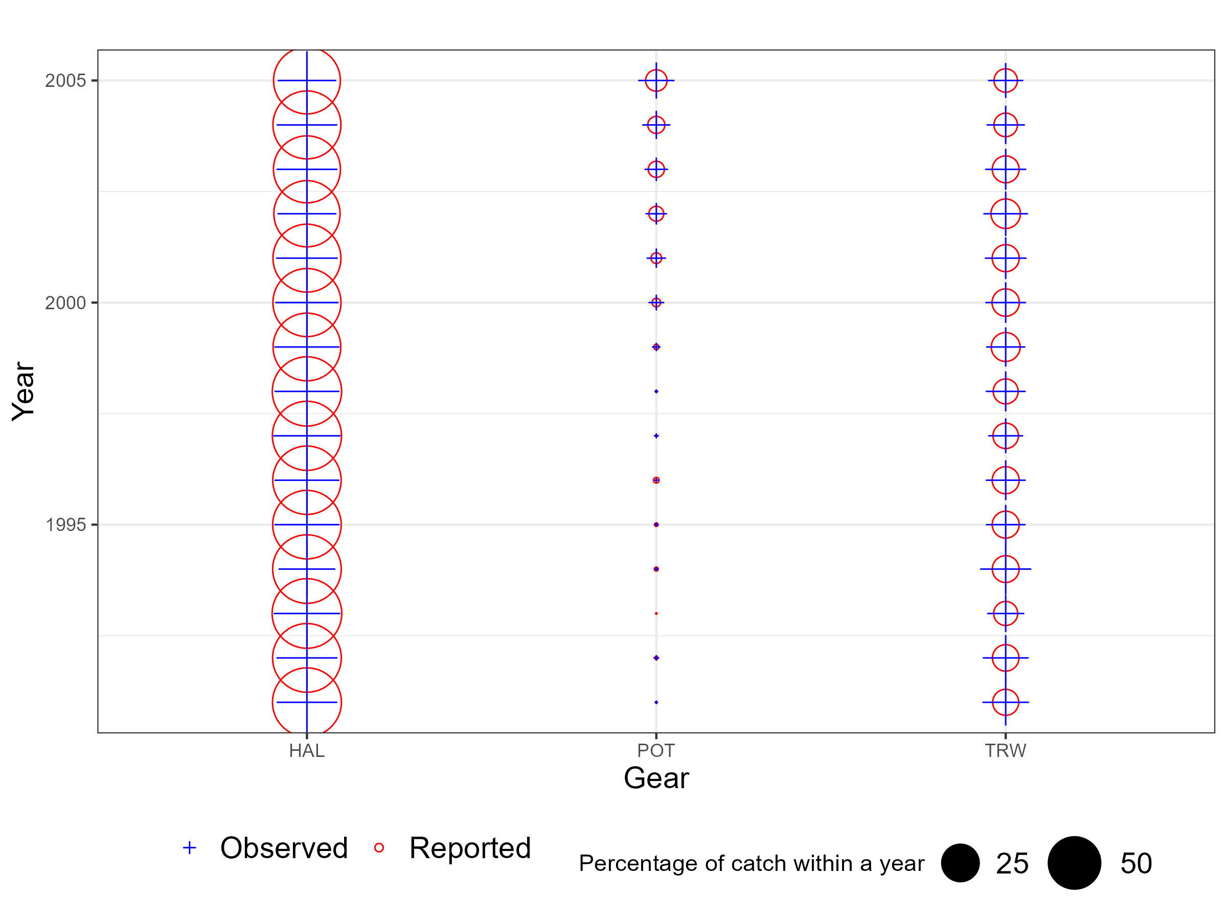
Figure 6.3: Observer representative figures by method. When the cross and circle are the same size this indicates observers sample proportional to the catch for a year.
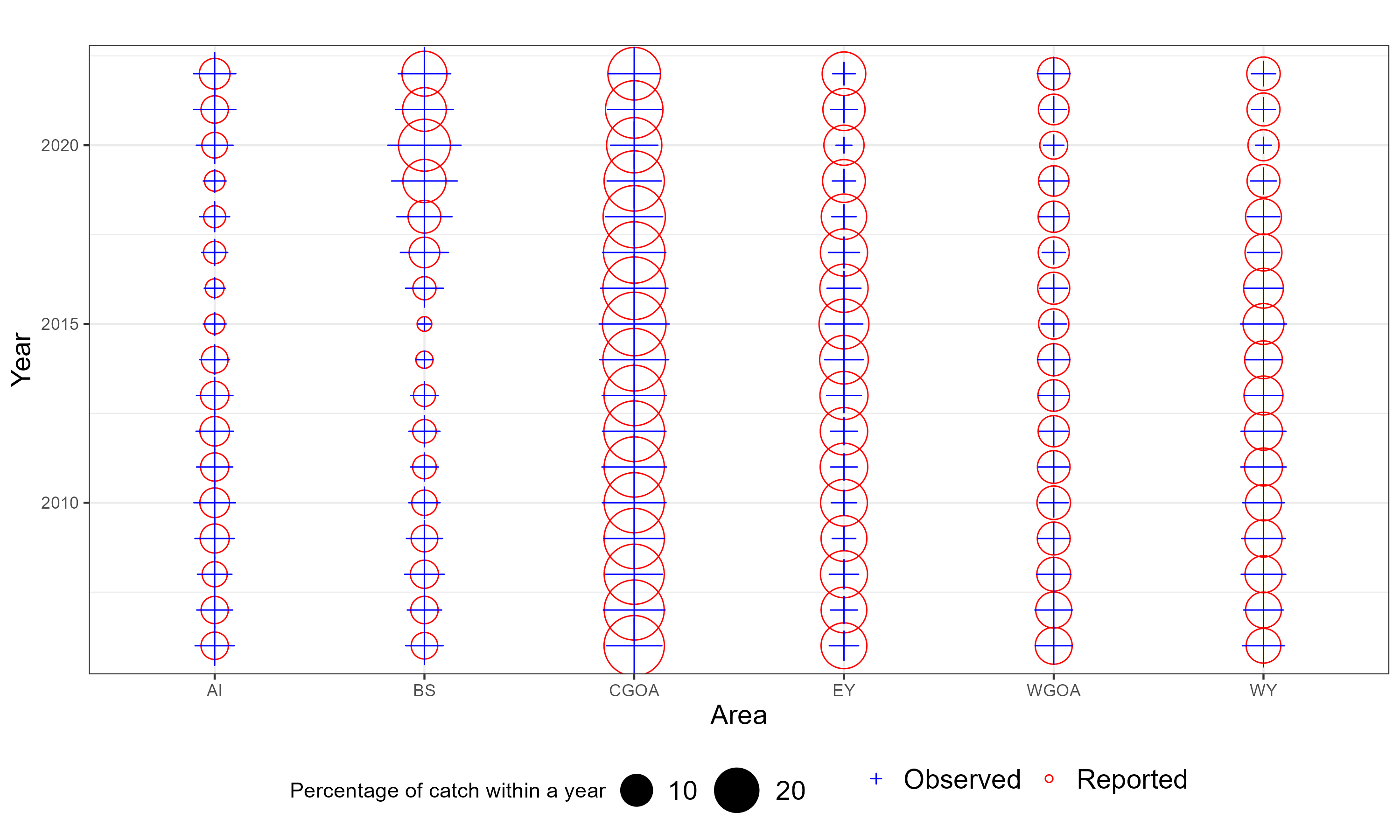
Figure 6.4: Observer representative figures by method. When the cross and circle are the same size this indicates observers sample proportional to the catch for a year.
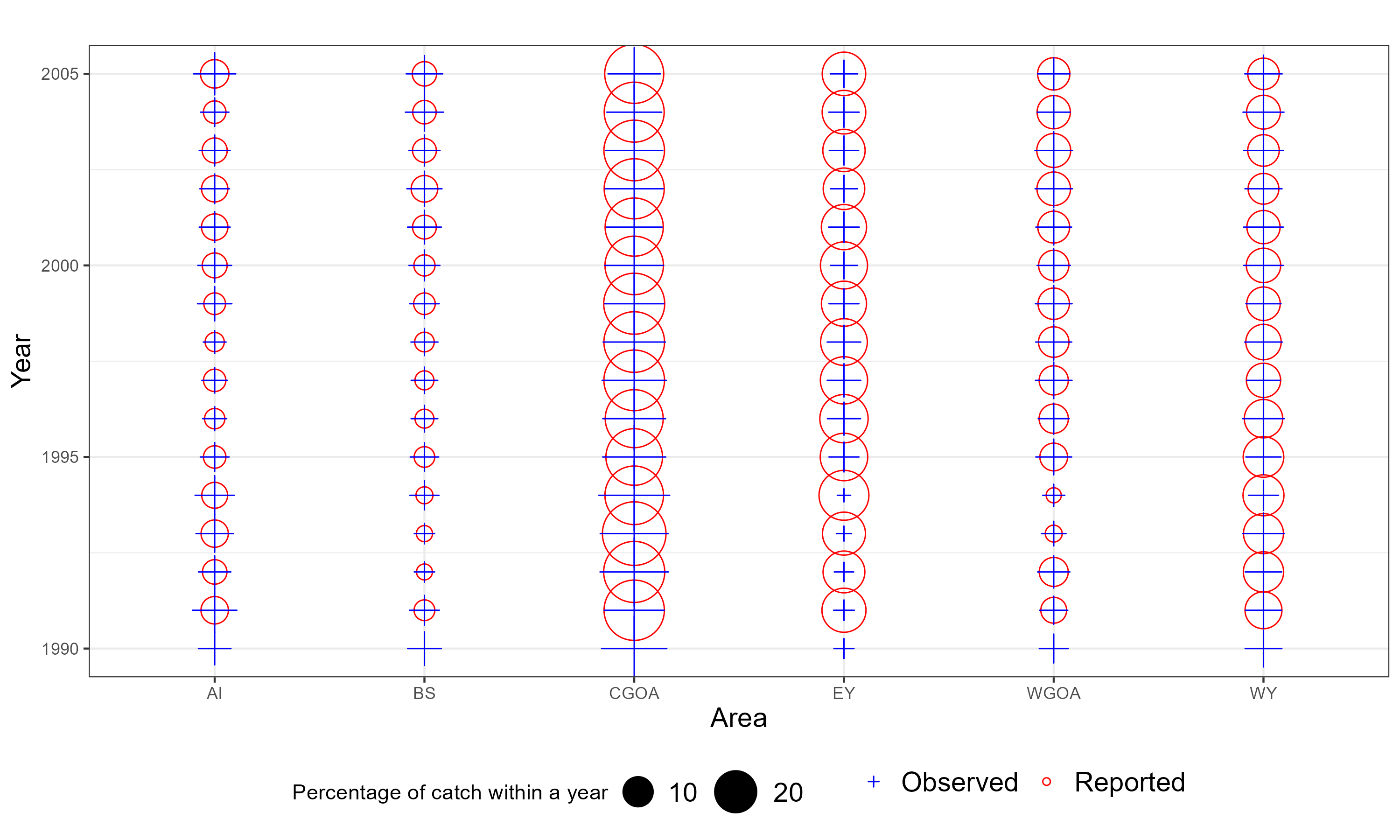
Figure 6.5: Observer representative figures by method. When the cross and circle are the same size this indicates observers sample proportional to the catch for a year.
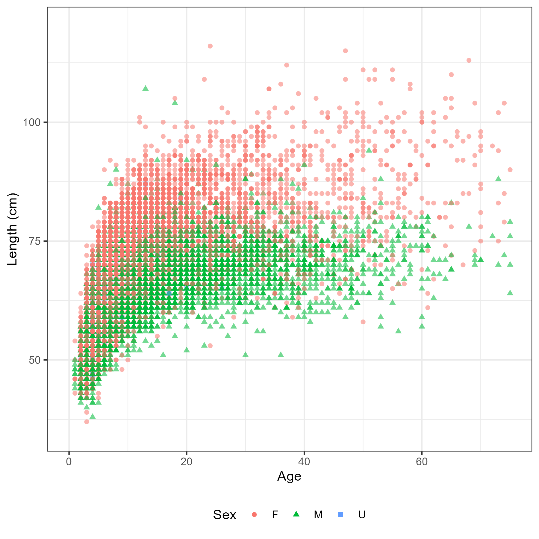
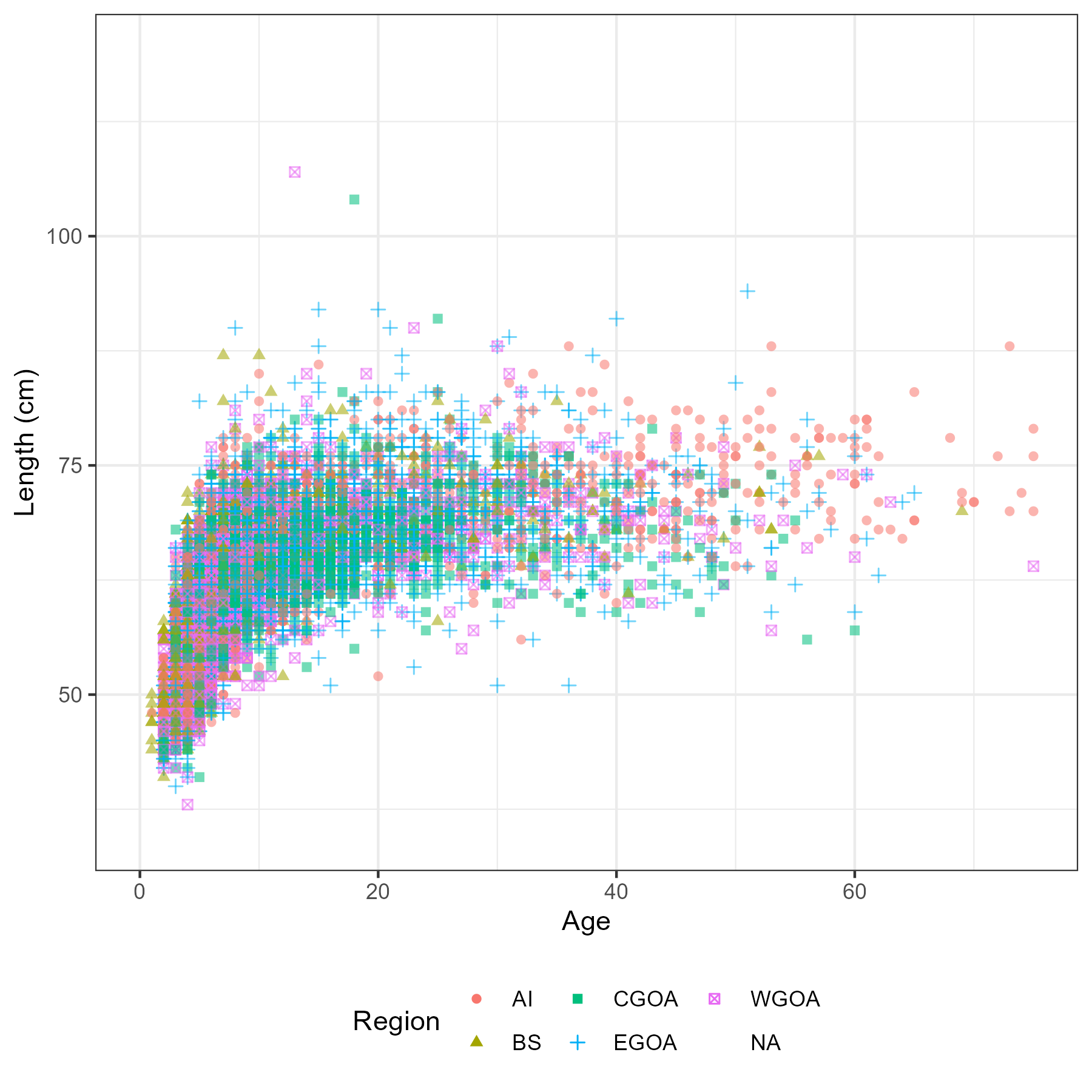
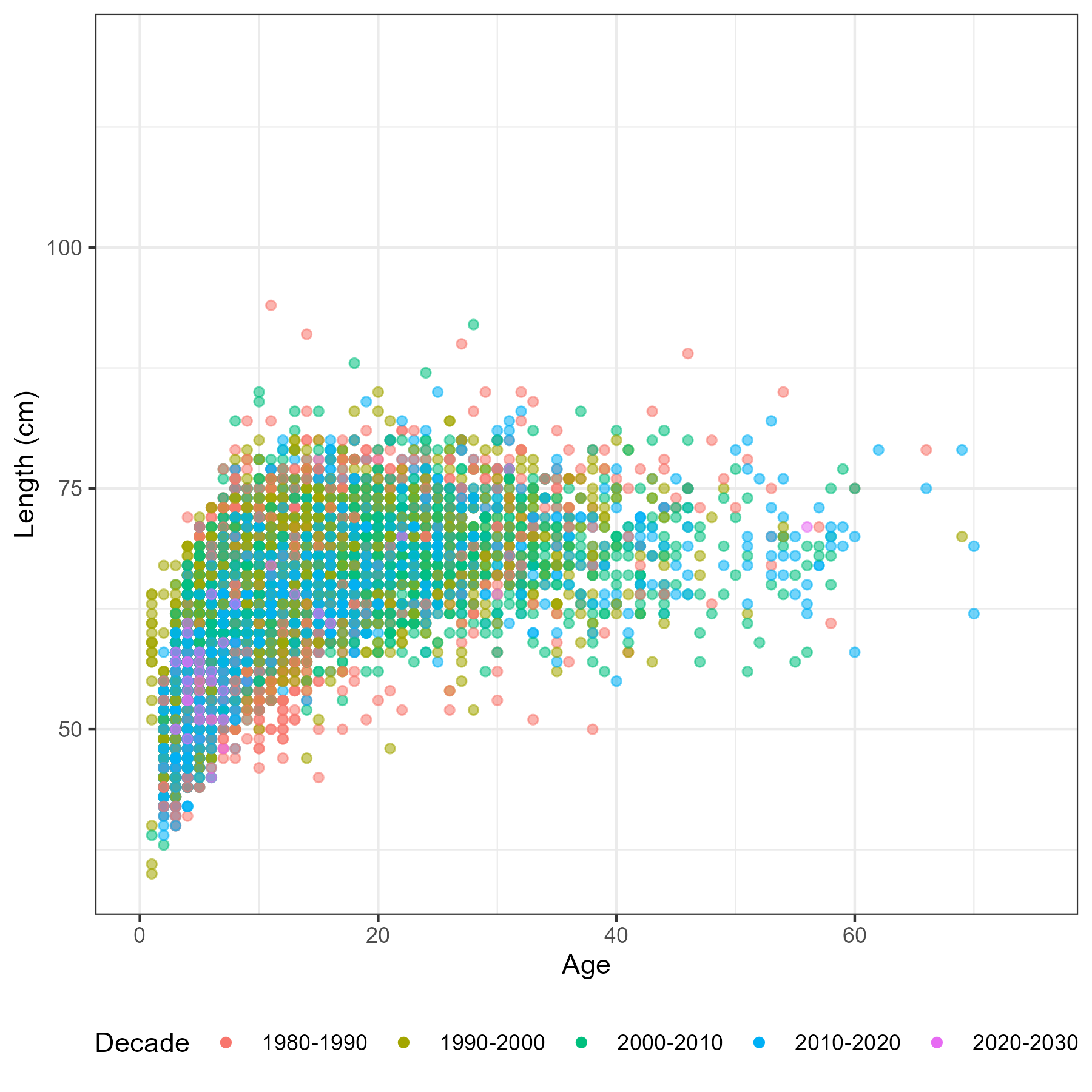
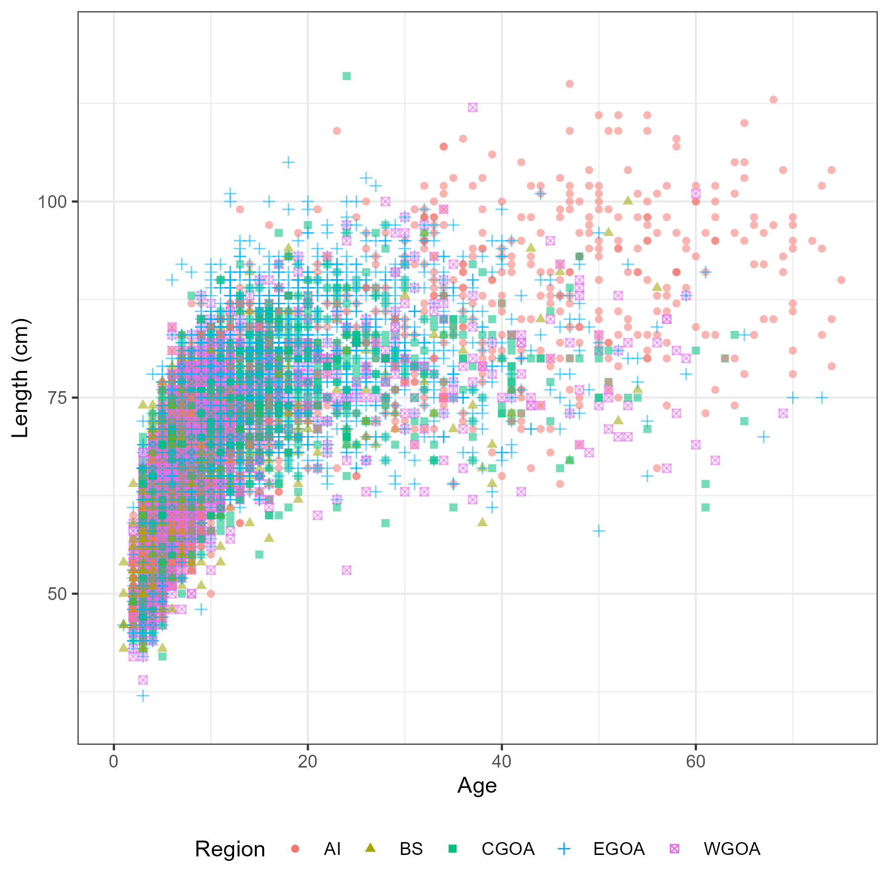
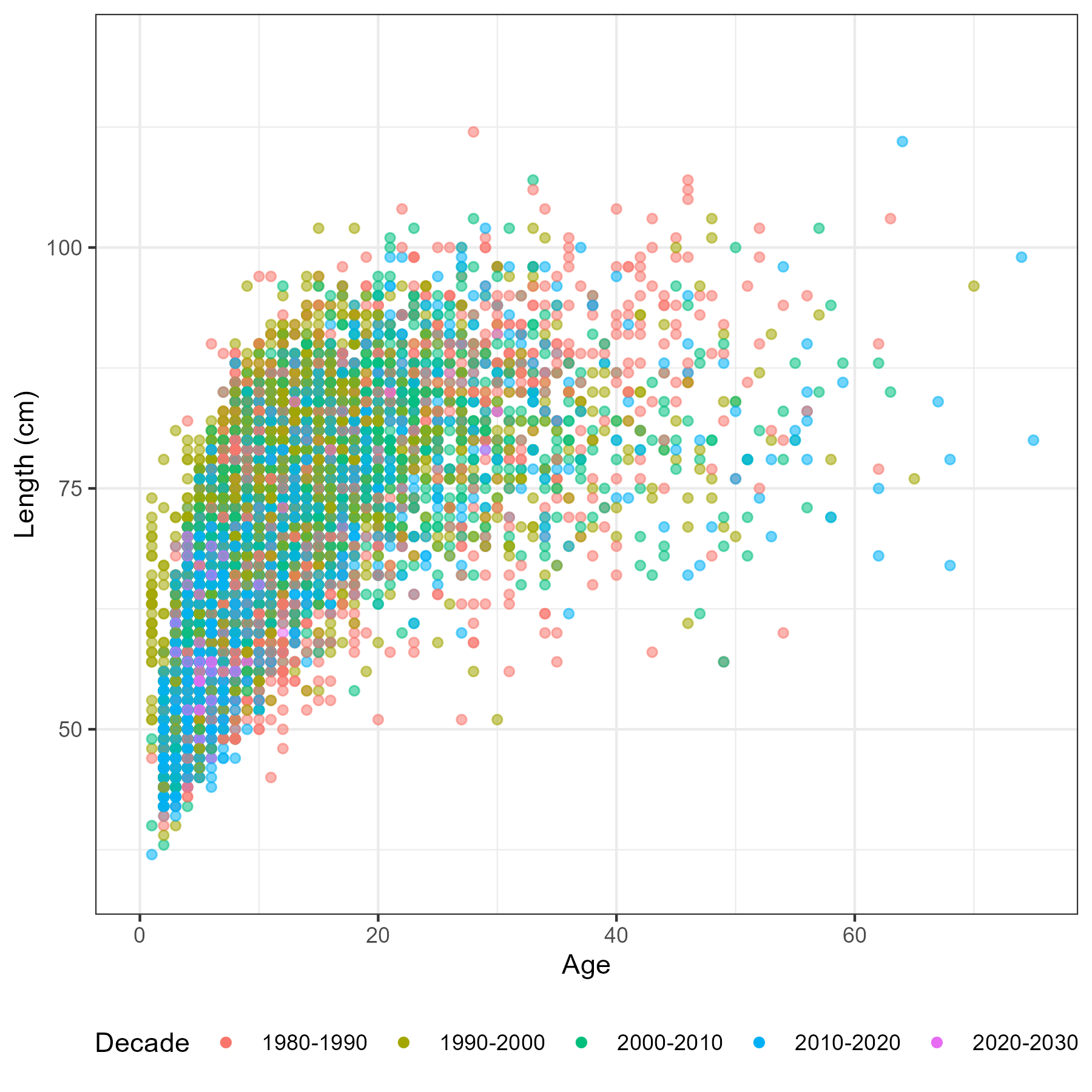
Length data
Catch at length estimator
The aim of catch at length is to obtain representative length frequencies (LF) of fish removed by a specific fishery within a specific area and year. These estimates are derived from observer collected data of which only a subsample of fishing trips are observed. Observers are tasked with subsampling observed catch to provide length and age samples. Thus these samples need to be scaled to either the stock wide level for inputs into a single area stock assessment or to some region level for use in a spatially disaggregated stock assessment. This is sampling structure has a natural hierarchy which is illustrated in Figure 6.6.
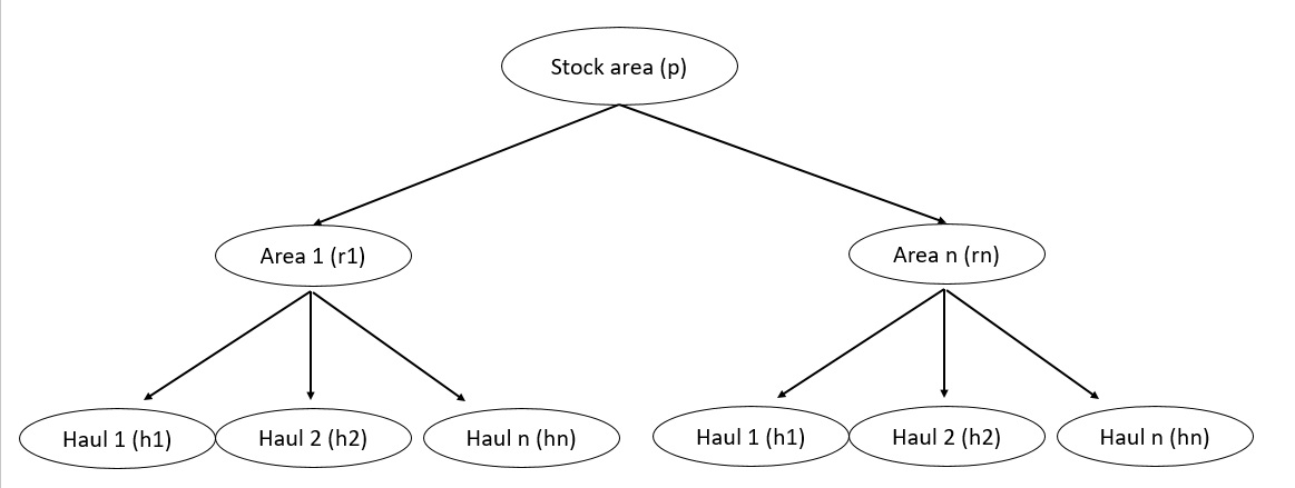
Figure 6.6: Sampling hierachy for fishery dependent catch at age and catch at length estimates
Each node in the sampling hierarchy is denoted by the index \(m\). When a node is nested within another node, we use \(m \in m'\) to define that \(m'\) is nested within \(m\).
| Symbol | Description |
|---|---|
| \(m,l,a,s\) | index for node, length bin, age bin, sex |
| \(n_{m,l,s},N_{m,l,s}\) | Number of fish in unscaled and scaled LF for sex \(s\), at node \(m\) |
| \(n_{m,a,s},N_{m,a,s}\) | Number of fish in unscaled and scaled AF for sex \(s\), at node \(m\) |
| \(q_m\) | Number of child nodes for node \(m\) |
| \(n_{m,l,a,s},N_{m,l,a,s}\) | Number of fish in unscaled and scaled LF & AF for sex \(s\), at node \(m\) |
| \(\pi_m\) | Scaling factor at node \(m\) |
| \(W_m,M_m,P_m,A_m\) | scaling variables for each node (weight, numbers, proportion, area) |
| \(w_{l,s}\) | mean weight for length bin \(l\) and sex \(s\) |
| \(w_{a,s}\) | mean weight for age bin \(a\) and sex \(s\) |
| \(K_{m,l,a,s}\) | Age-length key for node \(m\) by sex |
We require information the numbers at length for each node ( \(n_{m,l,s}\)) which make up the unscaled length frequency. Length weight parameters that describe the allometric relationship of weight from length (\(w_{l,s} = a_s L_{l,s}^{b_s}\)). The last piece is how we want to scale the frequencies (\(W_m,M_m,P_m,A_m\)). Length frequencies are iteratively calculated up the sampling hierarchy
\[ n_{m,l,s} = \sum_{m' \in m} N_{m',l,s} \] where \[ N_{m',l,s} = \pi_{m'} n_{m',l,s} \]
There are multiple approaches for scaling unscaled numbers to scaled numbers such as scaling by area etc, scaling by weight.
If an individual haul is subsampled i.e., only 50 fish are measured for length of 1000 caught in a single haul, then we use the sampling fraction denoted by \(\pi^{h}\) to scale the subsample to a haul level LF. Region wide LFs are calculated by summing the LFs over all sampled hauls within that region. Due to each haul having a scaled LF hauls, hauls with larger catches will naturally contribute more samples to a region wide LF, thus making this a catch weighted estimator.
If \(n^h_l\) fish are measured for lengths from a haul that had \(N^h_l\) fish, then the scaler for the subsample follows, \[ \pi^{h} = \frac{N^h_l}{n^h_l} \] each length sample in haul \(h\) is divided by this sampling fraction.
The estimator for region wide LFs denoted by \(\widehat{N}^r_{l,s}\) follow,
\[ \widehat{N}^r_{l,s} = \sum_{h\in a} n^h_{l,s} \pi^{h} \pi^{r} \] where \(\pi^{r}\), is the region scalar which weights each observed haul by the catch from hauls that had LFs collected and total catch in the region. \[ \pi^{r} = \frac{C_r}{\sum_{h \in h'} C_h} \] where, \(C_h\) is the catch from haul \(h\), \(h'\) denotes the set of hauls that were observed and had LFs taken, and \(C_r\) is the region wide catch, which is a legal requirement from fishers to report.
Region wide LFs are aggregated across multiple regions denoted by the set \(r'\) using an another catch weighted approach
\[ \widehat{N}^{r'}_{l,s} = \sum_{r\in r'} \widehat{N}^r_{l,s} \pi^{r} \] where,
\[ \pi^{r} = \frac{C_r}{\sum_r C_r} \] where, \(A_r\) is the catch in region \(C_r\) and \(\sum_r C_r\) denotes catch over all regions under investigation.
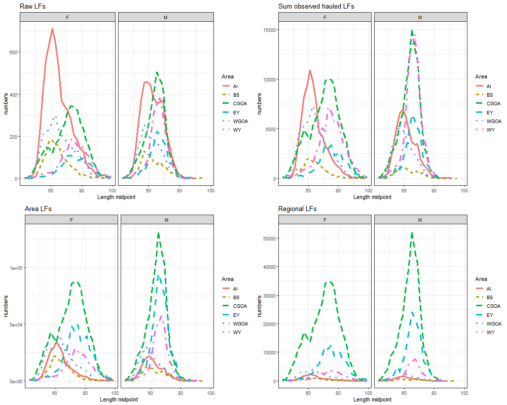
Figure 6.7: This figure shows how each of the scaling factors change the raw sampled LFs (\(n^h_{l,s}\)) to obtain regional scaled length frequencies (\(\widehat{N}^{r'}_{l,s}\)) for the fixed gear fishery.
A gear and region had to have at least 100 fish measured for length in order to generate catch at length estimates.